Chapter 5: The Box-Jenkins Methodology

1 Introduction

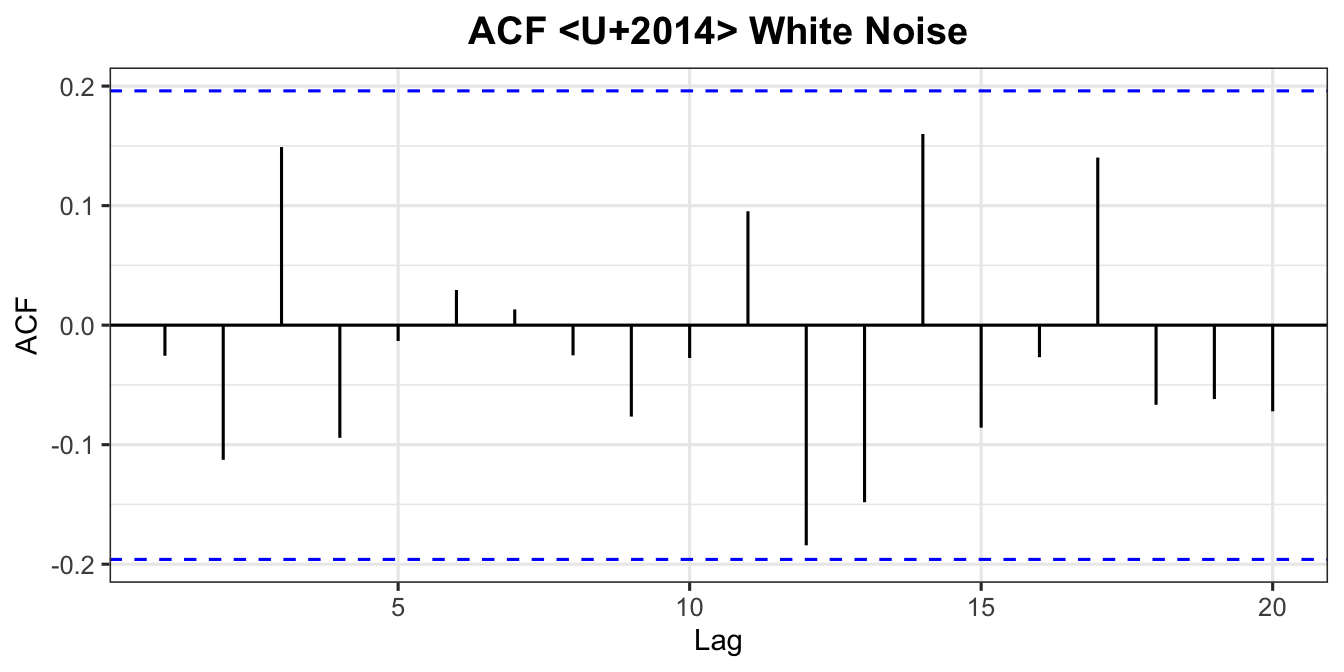
The ARIMA (AutoRegressive Integrated Moving Average) model is one of the most widely used statistical methods for time series forecasting. The Box-Jenkins methodology — developed by George Box and Gwilym Jenkins — provides a systematic four-stage approach for identifying, estimating, validating, and applying ARIMA models.

Four basic model types are involved:

Model	Acronym	Description
Autoregressive	AR	Current value depends on its own past values
Moving Average	MA	Current value depends on past error terms
Mixed Autoregressive and Moving Average	ARMA	Combination of AR and MA
Mixed Autoregressive Integrated Moving Average	ARIMA	ARMA applied to differenced series

2 ARIMA Models

2.1 Autoregressive (AR) Model

A $p$th-order autoregressive model, AR($p$), is:

\[ y_t = \phi_0 + \phi_1 y_{t-1} + \phi_2 y_{t-2} + \cdots + \phi_p y_{t-p} + \varepsilon_t \tag{1} \]

where:

$y_t$ = the response variable at time $t$
$y_{t-1}, y_{t-2}, \ldots, y_{t-p}$ = the response variable at lags $1, 2, \ldots, p$ (acting as independent variables)
$\phi_0, \phi_1, \ldots, \phi_p$ = coefficients to be estimated
$\varepsilon_t$ = error term at time $t$

Using the backward shift operator $B$, Equation (1) becomes:

\[ (1 - \phi_1 B - \phi_2 B^2 - \cdots - \phi_p B^p)\,y_t = \phi_0 + \varepsilon_t \]

2.1.1 AR(1) — the simplest form

\[ y_t = \phi_0 + \phi_1 y_{t-1} + \varepsilon_t \tag{2} \]

\[ \Rightarrow (1 - \phi_1 B)\,y_t = \phi_0 + \varepsilon_t \tag{3} \]

The current value at time $t$ equals the mean plus a contribution from one period back, plus the error term.

2.2 Moving Average (MA) Model

A $q$th-order moving average model, MA($q$), is:

\[ y_t = \phi_0 + \varepsilon_t + \theta_1 \varepsilon_{t-1} + \theta_2 \varepsilon_{t-2} + \cdots + \theta_q \varepsilon_{t-q} \tag{4} \]

where:

$\phi_0$ = constant mean of the process
$\theta_1, \theta_2, \ldots, \theta_q$ = MA coefficients to be estimated
$\varepsilon_t, \varepsilon_{t-1}, \ldots$ = current and past error terms

In backshift notation:

\[ y_t = \phi_0 + (1 + \theta_1 B + \theta_2 B^2 + \cdots + \theta_q B^q)\,\varepsilon_t \]

2.2.1 MA(1) — the simplest form

\[ y_t = \phi_0 + \theta_1 \varepsilon_{t-1} + \varepsilon_t \tag{5} \]

\[ \Rightarrow y_t = \phi_0 + (1 + \theta_1 B)\,\varepsilon_t \]

2.3 Mixed Autoregressive Moving Average — ARMA($p$,$q$)

ARMA($p,q$) combines AR order $p$ and MA order $q$:

\[ y_t = \phi_0 + \phi_1 y_{t-1} + \cdots + \phi_p y_{t-p} + \varepsilon_t + \theta_1 \varepsilon_{t-1} + \cdots + \theta_q \varepsilon_{t-q} \tag{6} \]

In backshift notation:

\[ (1 - \phi_1 B - \cdots - \phi_p B^p)\,y_t = \phi_0 + (1 + \theta_1 B + \cdots + \theta_q B^q)\,\varepsilon_t \tag{7} \]

2.3.1 ARMA(1,1) — the simplest form

\[ y_t = \phi_0 + \phi_1 y_{t-1} + \theta_1 \varepsilon_{t-1} + \varepsilon_t \]

\[ \Rightarrow (1 - \phi_1 B)\,y_t = \phi_0 + (1 + \theta_1 B)\,\varepsilon_t \]

2.4 Autoregressive Integrated Moving Average — ARIMA($p$,$d$,$q$)

When the stationarity assumption is not fulfilled, the series must be differenced $d$ times to achieve stationarity. The resulting model is ARIMA($p,d,q$).

2.4.1 ARIMA(1,1,1) — a simple case

Let $w_t = y_t - y_{t-1}$ (first difference, assumed stationary). Then:

\[ w_t = \phi_0 + \phi_1 w_{t-1} + \theta_1 \varepsilon_{t-1} + \varepsilon_t \tag{8} \]

\[ (1 - \phi_1 B)\,w_t = \phi_0 + (1 + \theta_1 B)\,\varepsilon_t \tag{9} \]

Setting $\phi_0 = 0$ and substituting $w_t = (1 - B)y_t$:

\[ (1 - \phi_1 B)(1 - B)\,y_t = (1 + \theta_1 B)\,\varepsilon_t \]

Expanding both sides:

\[ y_t - y_{t-1} - \phi_1 y_{t-1} + \phi_1 y_{t-2} = \varepsilon_t + \theta_1 \varepsilon_{t-1} \tag{10} \]

Solving for $y_t$:

\[ y_t = (1 + \phi_1) y_{t-1} - \phi_1 y_{t-2} + \varepsilon_t + \theta_1 \varepsilon_{t-1} \tag{11} \]

Note

Equation (11) resembles ARIMA(2,0,1), but it remains ARIMA(1,1,1) — the coefficients do not independently satisfy stationarity conditions for a second-order AR model.

Tip

Exercise: Write the backward shift operator formulations for:

ARIMA(2,1,2)
ARIMA(1,2,2)

2.5 Seasonal ARIMA — SARIMA($p$,$d$,$q$)($P$,$D$,$Q$)$_s$

For series exhibiting a seasonal component, seasonal differencing is required to remove the seasonality effect.

Let $z_t$ be the seasonally differenced series:

\[ z_t = y_t - y_{t-12} \quad \text{(monthly)} \qquad z_t = y_t - y_{t-4} \quad \text{(quarterly)} \]

If $z_t$ is still not stationary, apply regular differencing: $w_t = z_t - z_{t-1}$.

General SARIMA notation: $\text{SARIMA}(p,d,q)(P,D,Q)_s$

Parameter	Meaning
$p$	Non-seasonal AR order
$d$	Non-seasonal differencing order
$q$	Non-seasonal MA order
$P$	Seasonal AR order
$D$	Seasonal differencing order
$Q$	Seasonal MA order
$s$	Length of seasonal period

Example: ARIMA$(1,1,1)(1,1,1)_{12}$: $p=1$, $d=1$, $q=1$ (non-seasonal); $P=1$, $D=1$, $Q=1$ (seasonal); $s=12$ (monthly data).

2.5.1 Formulating SARIMA$(1,1,2)(1,1,1)_4$

Step 1 — Non-seasonal part ARIMA(1,1,2):

\[ (1 - \phi_1 B)(1 - B)(1 - B^4)\,y_t = (1 + \theta_1 B + \theta_2 B^2)\,\varepsilon_t \]

Step 2 — Seasonal part SARIMA(1,1,1):

\[ (1 - \Phi_1 B^4)(1 - B^4)\,y_t = (1 + \Theta_1 B^4)\,\varepsilon_t \]

Step 3 — Combined model:

\[ (1 - \phi_1 B)(1 - B)(1 - \Phi_1 B^4)(1 - B^4)\,y_t = (1 + \theta_1 B + \theta_2 B^2)(1 + \Theta_1 B^4)\,\varepsilon_t \]

Tip

Exercise: Write the backward shift operator formulations for:

SARIMA$(2,1,1)(1,1,1)_4$
SARIMA$(2,1,2)(2,1,2)_{12}$

3 Box-Jenkins Methodology: Overview

The Box-Jenkins methodology involves four iterative stages:

Stage	Name	Description
1	Model Identification	Use ACF/PACF and ADF test to determine $p$, $d$, $q$
2	Model Estimation	Estimate parameters using OLS or MLE
3	Model Validation	Check residuals for white noise (Ljung-Box, AIC, BIC)
4	Model Application	Generate forecasts from the best model

If validation fails, return to Stage 1 and revise the model.

General identification rules:

Data fluctuates around a constant value → ARMA($p,q$)
Data has a trend → first-order differencing → ARIMA($p,d,q$)
Data has a seasonal component → seasonal differencing → SARIMA$(p,d,q)(P,D,Q)_s$

4 Autocorrelation Function (ACF)

4.1 Definition

The ACF measures the linear correlation between observations separated by lag $k$:

\[ r_k = \frac{\text{Cov}(y_t,\, y_{t+k})}{\sqrt{\text{Var}(y_t)\,\text{Var}(y_{t+k})}} \tag{12} \]

At lag 1:

\[ r_1 = \frac{\text{Cov}(y_t,\, y_{t+1})}{\sqrt{\text{Var}(y_t)\,\text{Var}(y_{t+1})}} \tag{13} \]

Under stationarity, $\text{Var}(y_t) = \text{Var}(y_{t-k}) = \sigma^2$, so:

\[ r_k = \frac{\text{Cov}(y_t,\, y_{t+k})}{\text{Var}(y_t)} \tag{14} \]

The approximate 95% confidence band for each ACF coefficient is:

\[ r_k \pm \frac{1.96}{\sqrt{T}} \tag{15} \]

4.2 ACF of a Random Process (White Noise)

For $y_t = \phi_0 + \varepsilon_t$ with $\varepsilon_t \overset{iid}{\sim} (0, \sigma_\varepsilon^2)$, setting $\phi_0 = 0$:

At lag 0:

\[ r_0 = \frac{E(\varepsilon_t^2)}{\sigma_\varepsilon^2} = 1 \]

At lag $k > 0$:

\[ r_k = \frac{E(\varepsilon_t\,\varepsilon_{t+k})}{\sigma_\varepsilon^2} = 0 \quad \text{(errors are independent)} \]

All autocorrelations at lags $k > 0$ are zero. A white noise ACF shows all spikes within the confidence bounds.

Show R Code

set.seed(123)
e <- rnorm(100, mean = 0, sd = 1)
ggAcf(e, lag.max = 20) +
  labs(title = "ACF — White Noise") +
  theme_ts()

Figure 1: ACF of a white noise (random process) series. All spikes lie within the 95% confidence bands — no significant autocorrelation at any lag.

4.3 ACF of an AR(1) Process

From Chapter 4, for $y_t = \phi_1 y_{t-1} + \varepsilon_t$ (with $\phi_0 = 0$):

Multiplying both sides by $y_{t-k}$ and taking expectations:

\[ \gamma_1 = \phi_1\,\gamma_0 \implies r_1 = \phi_1 \]

In general, by the Yule-Walker equations:

\[ \gamma_k = \phi_1^k\,\gamma_0 \implies r_k = \phi_1^k \tag{16} \]

Pattern:

If $\phi_1 > 0$: ACF decays exponentially toward zero
If $\phi_1 < 0$: ACF decays exponentially with alternating signs

Show R Code

set.seed(111)
ar1_pos <- arima.sim(model = list(order = c(1,0,0), ar =  0.7), n = 100)
ar1_neg <- arima.sim(model = list(order = c(1,0,0), ar = -0.7), n = 100)

p_pos <- ggAcf(ar1_pos, lag.max = 20) +
  labs(title = expression(phi[1] == 0.7 ~ " (positive)")) + theme_ts()
p_neg <- ggAcf(ar1_neg, lag.max = 20) +
  labs(title = expression(phi[1] == -0.7 ~ " (negative)")) + theme_ts()

grid.arrange(p_pos, p_neg, ncol = 2)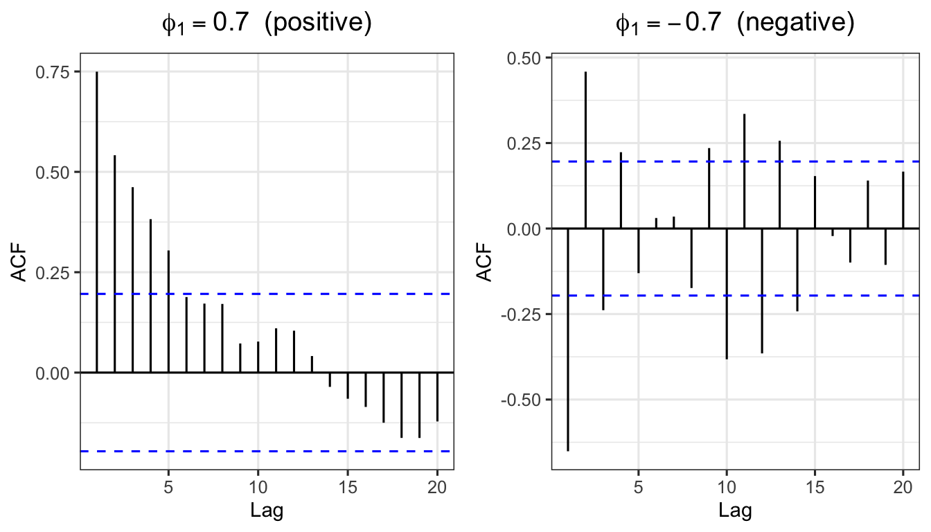

Figure 2: ACF for AR(1) with positive $\phi_1 = 0.7$ (left) and negative $\phi_1 = -0.7$ (right). Positive $\phi_1$ gives smooth exponential decay; negative $\phi_1$ gives alternating decay.

Example: For AR(1) with $\phi_1 = 0.7$, theoretical ACF values:

\[r_1 = 0.7^1 = 0.700, \quad r_2 = 0.7^2 = 0.490, \quad r_3 = 0.7^3 = 0.343, \quad \ldots\]

Tip

Exercise for AR(2): For $y_t = \phi_0 + \phi_1 y_{t-1} + \phi_2 y_{t-2} + \varepsilon_t$, prove that:

\[r_1 = \frac{\phi_1}{1 - \phi_2}, \qquad r_2 = \frac{\phi_1^2 + \phi_2(1+\phi_2)}{1-\phi_2}\]

4.4 ACF of an MA(1) Process

For $y_t = \phi_0 + \theta_1 \varepsilon_{t-1} + \varepsilon_t$:

\[ \text{Var}(y_t) = \gamma_0 = (1 + \theta_1^2)\,\sigma_\varepsilon^2 \]

\[ \gamma_1 = \theta_1\,\sigma_\varepsilon^2 \tag{17} \]

\[ \gamma_k = 0 \quad \text{for } k \geq 2 \]

Hence:

\[ r_1 = \frac{\theta_1}{1 + \theta_1^2}, \qquad r_k = 0 \text{ for } k \geq 2 \tag{18} \]

Pattern: ACF has exactly $q$ significant spikes (cuts off after lag $q$).

Example: MA(1) with $\theta_1 = 0.7$:

\[r_1 = \frac{0.7}{1 + 0.7^2} = \frac{0.7}{1.49} = 0.4698 \tag{19}\]

Show R Code

set.seed(111)
ma1 <- arima.sim(model = list(order = c(0,0,1), ma = 0.7), n = 100)
ggAcf(ma1, lag.max = 20) +
  labs(title = expression("ACF — MA(1), " ~ theta[1] == 0.7)) +
  theme_ts()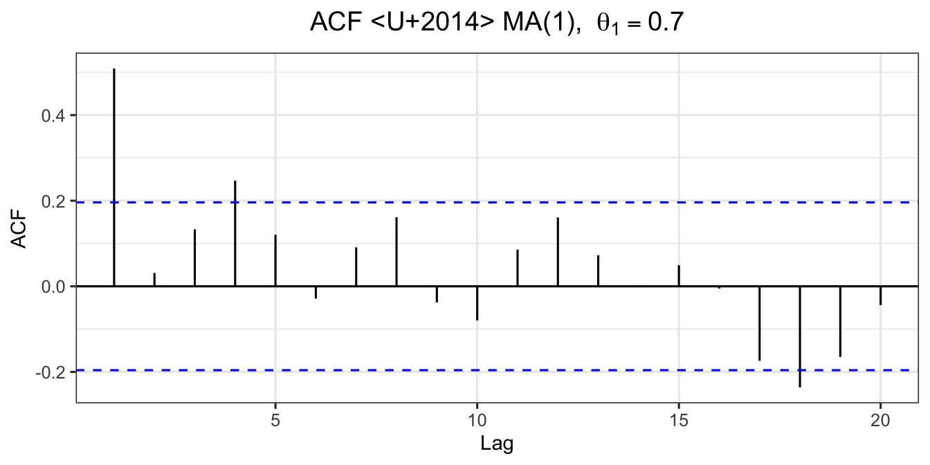

Figure 3: ACF for MA(1) with $\theta_1 = 0.7$. Only lag 1 is significant; all subsequent lags are within the confidence bands — the characteristic ‘cut-off’ pattern of a MA process.

Tip

Exercise for MA(2): For $y_t = \phi_0 + \theta_1\varepsilon_{t-1} + \theta_2\varepsilon_{t-2} + \varepsilon_t$, prove that:

\[r_1 = \frac{\theta_1 + \theta_1\theta_2}{1 + \theta_1^2 + \theta_2^2}, \qquad r_2 = \frac{\theta_2}{1 + \theta_1^2 + \theta_2^2}\]

5 Partial Autocorrelation Function (PACF)

5.1 Definition

The PACF measures the correlation between $y_t$ and $y_{t-k}$ after removing the linear effects of the intermediate lags $y_{t-1}, y_{t-2}, \ldots, y_{t-k+1}$.

The PACF is computed iteratively via the Yule-Walker equations. The PACF at lag $k$, denoted $\alpha_k$, is:

\[ \alpha_k = \frac{r_k - \displaystyle\sum_{j=1}^{k-1} \phi_j^{(k-1)}\,r_{k-j}} {1 - \displaystyle\sum_{j=1}^{k-1} \phi_j^{(k-1)}\,r_j} \tag{20} \]

with the recursion $\phi_j^{(k)} = \phi_j^{(k-1)} - \alpha_k\,\phi_{k-j}^{(k-1)}$.

5.2 ACF and PACF Patterns — Model Identification Guide

Model	ACF	PACF	Example
AR($p$)	The coefficients show a decay pattern	There are $k$ significant spike(s)	If the PACF shows that there is one significant spike observed at lag 1 and ACF exhibits a decay pattern, the suggested model is AR(1).
MA($q$)	There are $k$ significant spike(s)	The coefficients show a decay pattern	If the ACF shows that there is one significant spike observed at lag 1 and PACF exhibits a decay pattern, the suggested model is MA(1).
ARMA($p$,$q$)	There are $k$ significant spike(s)	There are $k$ significant spike(s)	If the ACF shows that there is one significant spike observed at lag 1 and PACF shows that there is one significant spike observed at lag 1, the suggested model is ARMA(1,1).

5.2.1 Example: Constructing ACF and PACF Plots from a Table

For a time series with $T = 100$ observations, the sample ACF and PACF values at lags 1 to 7 are given as:

Lag	1	2	3	4	5	6	7
ACF	0.35	0.15	0.029	−0.04	−0.021	−0.11	−0.01
PACF	0.25	0.13	−0.012	−0.165	−0.018	−0.10	0.035

The 95% confidence band is:

\[\pm \frac{1.96}{\sqrt{T}} = \pm \frac{1.96}{\sqrt{100}} = \pm 0.196\]

Any spike that falls outside $\pm 0.196$ is considered statistically significant.

Show R Code

T_obs  <- 100
ci     <- 1.96 / sqrt(T_obs)   # ±0.196

lag_vals  <- 1:7
acf_vals  <- c(0.35, 0.15, 0.029, -0.04, -0.021, -0.11, -0.01)
pacf_vals <- c(0.25, 0.13, -0.012, -0.165, -0.018, -0.10, 0.035)

df_acf  <- data.frame(lag = lag_vals, value = acf_vals,
                      sig = abs(acf_vals)  > ci)
df_pacf <- data.frame(lag = lag_vals, value = pacf_vals,
                      sig = abs(pacf_vals) > ci)

p_acf_ex <- ggplot(df_acf, aes(x = lag, y = value, fill = sig)) +
  geom_bar(stat = "identity", width = 0.4, colour = "black", linewidth = 0.3) +
  geom_hline(yintercept =  ci, linetype = "dashed", colour = "steelblue") +
  geom_hline(yintercept = -ci, linetype = "dashed", colour = "steelblue") +
  geom_hline(yintercept =  0,  colour = "black",    linewidth = 0.4) +
  scale_fill_manual(values = c("TRUE" = "#d62728", "FALSE" = "grey60"),
                    guide = "none") +
  scale_x_continuous(breaks = lag_vals) +
  labs(title = "ACF", x = "Lag", y = "ACF") +
  theme_ts()

p_pacf_ex <- ggplot(df_pacf, aes(x = lag, y = value, fill = sig)) +
  geom_bar(stat = "identity", width = 0.4, colour = "black", linewidth = 0.3) +
  geom_hline(yintercept =  ci, linetype = "dashed", colour = "steelblue") +
  geom_hline(yintercept = -ci, linetype = "dashed", colour = "steelblue") +
  geom_hline(yintercept =  0,  colour = "black",    linewidth = 0.4) +
  scale_fill_manual(values = c("TRUE" = "#d62728", "FALSE" = "grey60"),
                    guide = "none") +
  scale_x_continuous(breaks = lag_vals) +
  labs(title = "PACF", x = "Lag", y = "PACF") +
  theme_ts()

grid.arrange(p_acf_ex, p_pacf_ex, ncol = 2)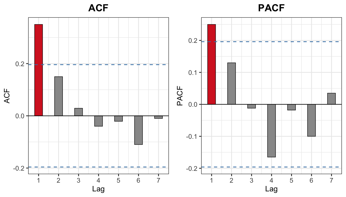

Figure 4: ACF (left) and PACF (right) plots constructed from the table of values for a 100-observation series. The dashed blue lines mark the 95% significance bounds (±0.196). Only lag 1 is significant in both plots, suggesting an ARMA(1,1) or possibly AR(1) model.

Interpretation:

ACF: Lag 1 (0.35) exceeds the bound of ±0.196 → significant. Lags 2–7 are within bounds → ACF cuts off after lag 1. This is consistent with an MA(1) pattern.
PACF: Lag 1 (0.25) exceeds the bound → significant. Lags 2–7 are within bounds → PACF cuts off after lag 1. This is consistent with an AR(1) pattern.
Both ACF and PACF show only one significant spike at lag 1 → the suggested model is ARMA(1,1).

Note

When both ACF and PACF show $k$ significant spikes at the same lags, the series is best described by an ARMA model. Here $k=1$ at lag 1, so ARMA(1,1) is the starting candidate.

Show R Code

set.seed(42)
sim_ar1   <- arima.sim(model = list(order=c(1,0,0), ar=0.7),           n=200)
sim_ma1   <- arima.sim(model = list(order=c(0,0,1), ma=0.7),           n=200)
sim_arma  <- arima.sim(model = list(order=c(1,0,1), ar=0.7, ma=0.5),   n=200)

p1 <- ggAcf(sim_ar1,  lag.max=20) + labs(title="AR(1) — ACF")  + theme_ts()
p2 <- ggPacf(sim_ar1, lag.max=20) + labs(title="AR(1) — PACF") + theme_ts()
p3 <- ggAcf(sim_ma1,  lag.max=20) + labs(title="MA(1) — ACF")  + theme_ts()
p4 <- ggPacf(sim_ma1, lag.max=20) + labs(title="MA(1) — PACF") + theme_ts()
p5 <- ggAcf(sim_arma,  lag.max=20) + labs(title="ARMA(1,1) — ACF")  + theme_ts()
p6 <- ggPacf(sim_arma, lag.max=20) + labs(title="ARMA(1,1) — PACF") + theme_ts()

grid.arrange(p1, p2, p3, p4, p5, p6, nrow=3)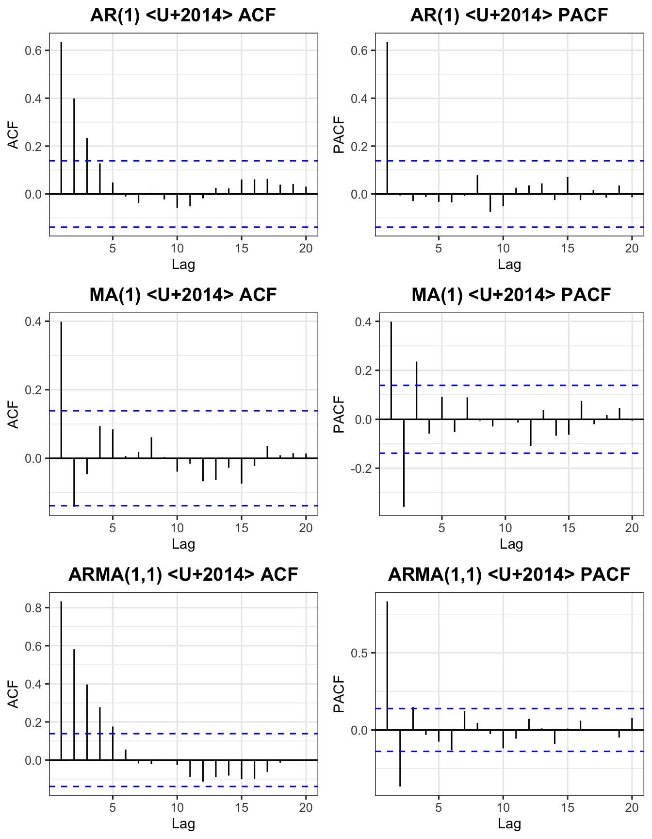

Figure 5: ACF (left column) and PACF (right column) patterns for AR(1) (top row), MA(1) (middle row), and ARMA(1,1) (bottom row). Note how the AR PACF cuts off at lag 1, the MA ACF cuts off at lag 1, and both plots tail off for ARMA.

6 Box-Jenkins: Non-Seasonal ARIMA

We demonstrate the full four-stage Box-Jenkins procedure using S&P 500 E-mini Futures (ES=F) daily adjusted close prices, April–December 2025, downloaded directly from Yahoo Finance via the quantmod package.

6.1 Stage 1 — Model Identification

6.1.1 Step 1a: Time Series Plot

Show R Code

autoplot(as.ts(est_snp)) +
  labs(title = "S&P 500 Futures (ES=F) — Estimation Set",
       subtitle = "Daily adjusted close price, Apr–Oct 2025",
       x = "Observation", y = "Price (USD)") +
  theme_ts()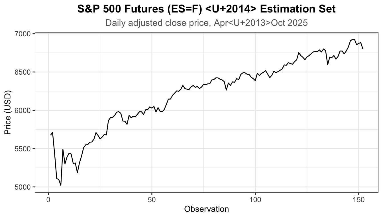

Figure 6: S&P 500 E-mini Futures (ES=F) daily adjusted close price, April–December 2025. The series wanders without a fixed mean — a sign of non-stationarity.

6.1.2 Step 1b: ACF and PACF of the Raw Series

Show R Code

p_acf_snp  <- ggAcf(est_snp,  lag.max = 30) +
  labs(title = "ACF — SNP Level") + theme_ts()
p_pacf_snp <- ggPacf(est_snp, lag.max = 30) +
  labs(title = "PACF — SNP Level") + theme_ts()
grid.arrange(p_acf_snp, p_pacf_snp, ncol = 2)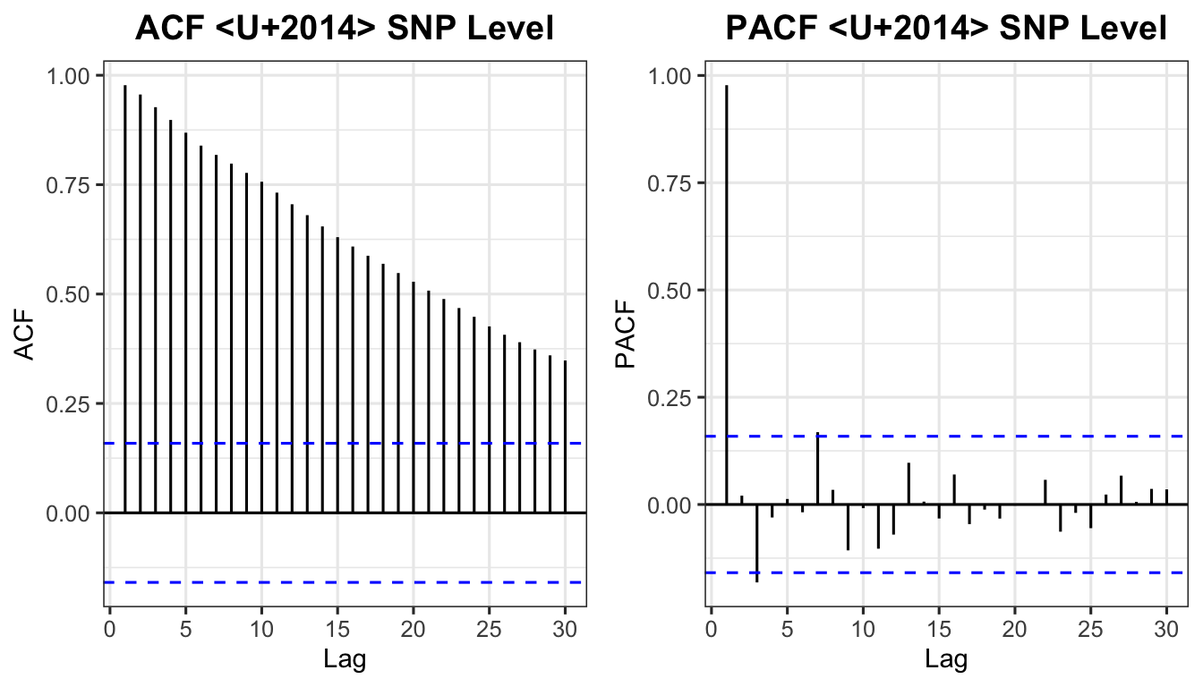

Figure 7: ACF (left) and PACF (right) of the raw S&P 500 price series. The ACF decays very slowly to zero — a clear sign of non-stationarity. First-order differencing is required.

6.1.3 Step 1c: ADF Test on Raw Series

Show R Code

adf.test(est_snp)


    Augmented Dickey-Fuller Test

data:  est_snp
Dickey-Fuller = -2.857, Lag order = 5, p-value = 0.2192
alternative hypothesis: stationary

Since $p$-value $> 0.05$, we fail to reject $H_0$ — the series is non-stationary.

6.1.4 Step 1d: First-Order Differencing

Show R Code

diff_snp <- diff(est_snp)

autoplot(as.ts(diff_snp)) +
  labs(title = "S&P 500 Futures — First Difference",
       subtitle = "Daily price changes",
       x = "Observation", y = expression(Delta ~ "Price")) +
  theme_ts()

Figure 8: S&P 500 first-differenced series (daily price changes). The series now fluctuates around a near-zero constant level — indicating stationarity.

Show R Code

adf.test(na.omit(diff_snp))


    Augmented Dickey-Fuller Test

data:  na.omit(diff_snp)
Dickey-Fuller = -6.1097, Lag order = 5, p-value = 0.01
alternative hypothesis: stationary

Since $p$-value $\leq 0.05$, we reject $H_0$ — the differenced series is stationary. Order of differencing: $d = 1$.

6.1.5 Step 1e: ACF and PACF of Differenced Series

Show R Code

p_acf_d  <- ggAcf(diff_snp,  lag.max = 30, na.action = na.omit) +
  labs(title = "ACF — First Difference") + theme_ts()
p_pacf_d <- ggPacf(diff_snp, lag.max = 30, na.action = na.omit) +
  labs(title = "PACF — First Difference") + theme_ts()
grid.arrange(p_acf_d, p_pacf_d, ncol = 2)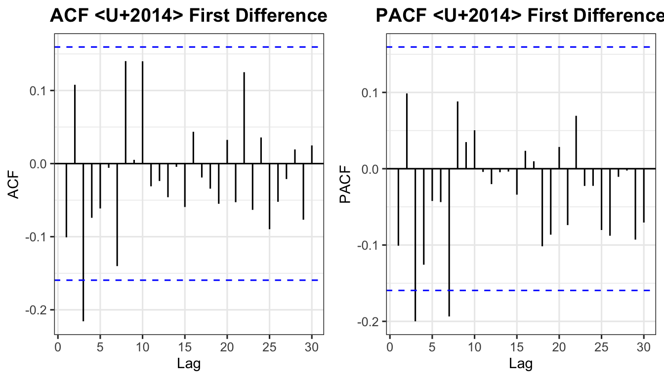

Figure 9: ACF (left) and PACF (right) of the first-differenced S&P 500 series. One significant spike at lag 3 on the ACF suggests MA(1); significant spikes at lags 3 and 8 on the PACF suggest AR(2). Suggested model: ARIMA(2,1,1).

Suggested model: ARIMA(2,1,1)

Competing models to compare: ARIMA(1,1,0) and ARIMA(2,1,2).

6.2 Stage 2 — Model Estimation (Non-Seasonal)

Show R Code

est_tbl <- as_tsibble(ts(as.numeric(est_snp)))
eva_tbl <- as_tsibble(ts(as.numeric(eva_snp)))

m211 <- est_tbl |> model(ARIMA(value ~ pdq(2,1,1)))
m110 <- est_tbl |> model(ARIMA(value ~ pdq(1,1,0)))
m212 <- est_tbl |> model(ARIMA(value ~ pdq(2,1,2)))

report(m211)

Series: value 
Model: ARIMA(2,1,1) 

Coefficients:
         ar1     ar2      ma1
      0.6848  0.0219  -0.7805
s.e.  0.2093  0.0947   0.1924

sigma^2 estimated as 5408:  log likelihood=-861.72
AIC=1731.45   AICc=1731.72   BIC=1743.52

Estimated equation for ARIMA(2,1,1):

\[ (1 - \hat\phi_1 B - \hat\phi_2 B^2)(1 - B)\,y_t = (1 + \hat\theta_1 B)\,\varepsilon_t \tag{21} \]

Tip

Exercise: Write the estimated equations for ARIMA(1,1,0) and ARIMA(2,1,2) using the coefficient values from report().

6.3 Stage 3 — Model Validation (Non-Seasonal)

6.3.1 Ljung-Box Test

The Ljung-Box statistic tests whether residuals are white noise:

\[ Q^*_{\text{calc}} = T(T+2)\sum_{k=1}^{h} \frac{r_k^2}{T-k} \tag{22} \]

approximately $\chi^2$ with $(h - p - q)$ degrees of freedom.

$H_0$: Residuals are white noise
$H_1$: Residuals are not white noise

If $p$-value $> 0.05$ → fail to reject $H_0$ → residuals are white noise → model is well-specified.

Show R Code

resid211 <- residuals(m211)
Box.test(resid211$.resid, lag = 20, type = "Ljung-Box", fitdf = 4)


    Box-Ljung test

data:  resid211$.resid
X-squared = 21.023, df = 16, p-value = 0.1776

Show R Code

p_ra  <- ggAcf(resid211$.resid,  lag.max = 20, na.action = na.omit) +
  labs(title = "Residual ACF")  + theme_ts()
p_rpa <- ggPacf(resid211$.resid, lag.max = 20, na.action = na.omit) +
  labs(title = "Residual PACF") + theme_ts()
grid.arrange(p_ra, p_rpa, ncol = 2)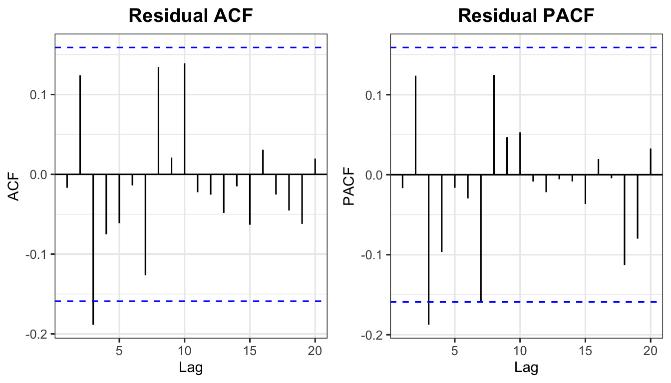

Figure 10: ACF and PACF of residuals from ARIMA(2,1,1) fitted to the S&P 500 estimation set. No significant spikes confirm the residuals are white noise.

6.3.2 Information Criteria

Akaike’s Information Criterion (AIC):

\[ \text{AIC} = -2\log(L) + 2(p + q + k + 1) \tag{23} \]

where $L$ is the likelihood, and $k = 1$ if $\phi_0 \neq 0$, else $k = 0$.

Corrected AIC (AICc):

\[ \text{AICc} = \text{AIC} + \frac{2(p+q+k+1)(p+q+k+2)}{T - p - q - k - 2} \tag{24} \]

Bayesian Information Criterion (BIC):

\[ \text{BIC} = \text{AIC} + [\log(T) - 2](p + q + k + 1) \tag{25} \]

Lower AIC / AICc / BIC = better model. BIC penalises complexity more heavily than AIC.

Show R Code

bind_rows(
  glance(m211) |> mutate(Model = "ARIMA(2,1,1)"),
  glance(m110) |> mutate(Model = "ARIMA(1,1,0)"),
  glance(m212) |> mutate(Model = "ARIMA(2,1,2)")
) |>
  select(Model, AIC, AICc, BIC) |>
  arrange(AIC)

# A tibble: 3 x 4
  Model          AIC  AICc   BIC
  <chr>        <dbl> <dbl> <dbl>
1 ARIMA(2,1,2) 1725. 1725. 1743.
2 ARIMA(1,1,0) 1728. 1728. 1734.
3 ARIMA(2,1,1) 1731. 1732. 1744.

The model with the lowest AIC/BIC is selected as the best model.

6.3.3 Parameter Redundancy

When two ARMA models produce the same series, they exhibit parameter redundancy. For example, a white noise process $y_t = \varepsilon_t$ can be rewritten as:

\[ y_t = -0.5\,y_{t-1} + \varepsilon_t + 0.5\,\varepsilon_{t-1} \tag{26} \]

which superficially resembles ARMA(1,1) but is not a genuinely different model. Always inspect ACF/PACF diagnostics to avoid over-parameterisation.

6.4 Stage 4 — Model Application: Forecasting (Non-Seasonal)

6.4.1 Three Steps for Point Forecasts

Expand the ARIMA equation so that $y_t$ is on the left-hand side.
Rewrite replacing $t$ with $T + h$.
On the right-hand side: replace future observations with their forecasts, future errors with zero, and past errors with corresponding residuals.

Example: ARIMA(1,1,1) forecast derivation

Expanded equation (from Equation 11):

\[ y_t = (1 + \phi_1)\,y_{t-1} - \phi_1\,y_{t-2} + \varepsilon_t + \theta_1\,\varepsilon_{t-1} \tag{27} \]

One-step-ahead forecast (substitute $t = T+1$, set $\varepsilon_{T+1} = 0$):

\[ \hat{y}_{T+1|T} = (1 + \hat\phi_1)\,y_T - \hat\phi_1\,y_{T-1} + \hat\theta_1\,\varepsilon_T \tag{28} \]

Two-step-ahead forecast ($\varepsilon_{T+2} = \varepsilon_{T+1} = 0$, replace $y_{T+1}$ with $\hat{y}_{T+1|T}$):

\[ \hat{y}_{T+2|T} = (1 + \hat\phi_1)\,\hat{y}_{T+1|T} - \hat\phi_1\,y_T \tag{29} \]

The process continues for all future periods $h = 3, 4, \ldots$

6.4.2 Forecast Exercise

Exercise

The price of S&P 500 futures (daily data, 190 observations, April 1 – December 31, 2025) was fitted with an ARIMA(2,1,1) model, producing the following output.

Model coefficients:

	ar1	ar2	ma1
Estimate	0.6848	0.0219	−0.7805
Std. Error	0.2093	0.0947	0.1924

Last three observations (fitted values and residuals):

Time	Price ($y_t$)	Fitted ($\hat{y}_t$)	Residual ($\varepsilon_t$)
Dec 29, 2025 (obs 188)	6,979.25	6,973.62	5.63
Dec 30, 2025 (obs 189)	6,955.00	6,973.10	−18.10
Dec 31, 2025 (obs 190)	6,944.25	6,952.45	−8.20

Prove that the S&P 500 forecast for January 1, 2026 (obs 191) and January 2, 2026 (obs 192) are 6,942.76 and 6,941.50 respectively.

Answer

Step 1 — Expand the ARIMA(2,1,1) equation

The ARIMA(2,1,1) model in differenced form is:

\[ (1 - \hat\phi_1 B - \hat\phi_2 B^2)(1-B)\,y_t = (1 + \hat\theta_1 B)\,\varepsilon_t \]

Expanding the left-hand side:

\[ (y_t - y_{t-1}) - \hat\phi_1(y_{t-1} - y_{t-2}) - \hat\phi_2(y_{t-2} - y_{t-3}) = \varepsilon_t + \hat\theta_1\,\varepsilon_{t-1} \]

Solving for $y_t$:

\[ y_t = (1+\hat\phi_1)\,y_{t-1} + (-\hat\phi_1+\hat\phi_2)\,y_{t-2} - \hat\phi_2\,y_{t-3} + \varepsilon_t + \hat\theta_1\,\varepsilon_{t-1} \tag{30} \]

With $\hat\phi_1 = 0.6848$, $\hat\phi_2 = 0.0219$, $\hat\theta_1 = -0.7805$:

\[ y_t = 1.6848\,y_{t-1} - 0.6629\,y_{t-2} - 0.0219\,y_{t-3} + \varepsilon_t - 0.7805\,\varepsilon_{t-1} \]

Step 2 — One-step-ahead forecast: $\hat{y}_{191|190}$ (January 1, 2026)

Substitute $t = T+1 = 191$. Set $\varepsilon_{T+1} = 0$ (future error unknown); replace past errors with residuals ($\varepsilon_T = -8.20$):

\[ \hat{y}_{191} = 1.6848\,y_{190} - 0.6629\,y_{189} - 0.0219\,y_{188} + \hat\theta_1\,\varepsilon_{190} \]

\[ = 1.6848 \times 6944.25 \;-\; 0.6629 \times 6955.00 \;-\; 0.0219 \times 6979.25 \;+\; (-0.7805)\times(-8.20) \]

\[ = 11{,}699.67 \;-\; 4{,}610.47 \;-\; 152.85 \;+\; 6.40 \]

\[ \boxed{\hat{y}_{191} = 6{,}942.76} \]

Step 3 — Two-step-ahead forecast: $\hat{y}_{192|190}$ (January 2, 2026)

Substitute $t = T+2 = 192$. Set $\varepsilon_{T+2} = \varepsilon_{T+1} = 0$; replace $y_{T+1}$ with $\hat{y}_{191} = 6{,}942.76$:

\[ \hat{y}_{192} = 1.6848\,\hat{y}_{191} - 0.6629\,y_{190} - 0.0219\,y_{189} \]

\[ = 1.6848 \times 6942.76 \;-\; 0.6629 \times 6944.25 \;-\; 0.0219 \times 6955.00 \]

\[ = 11{,}697.16 \;-\; 4{,}603.34 \;-\; 152.31 \]

\[ \boxed{\hat{y}_{192} = 6{,}941.50} \]

6.4.3 Forecast Plot

Show R Code

snp_tbl <- as_tsibble(ts(as.numeric(snp)))

m211_full <- snp_tbl |> model(ARIMA(value ~ pdq(2,1,1)))

m211_full |>
  forecast(h = 10) |>
  autoplot(snp_tbl, level = c(80, 95)) +
  labs(title = "S&P 500 Futures — ARIMA(2,1,1) 10-Step Forecast",
       x = "Observation", y = "Price (USD)") +
  theme_ts()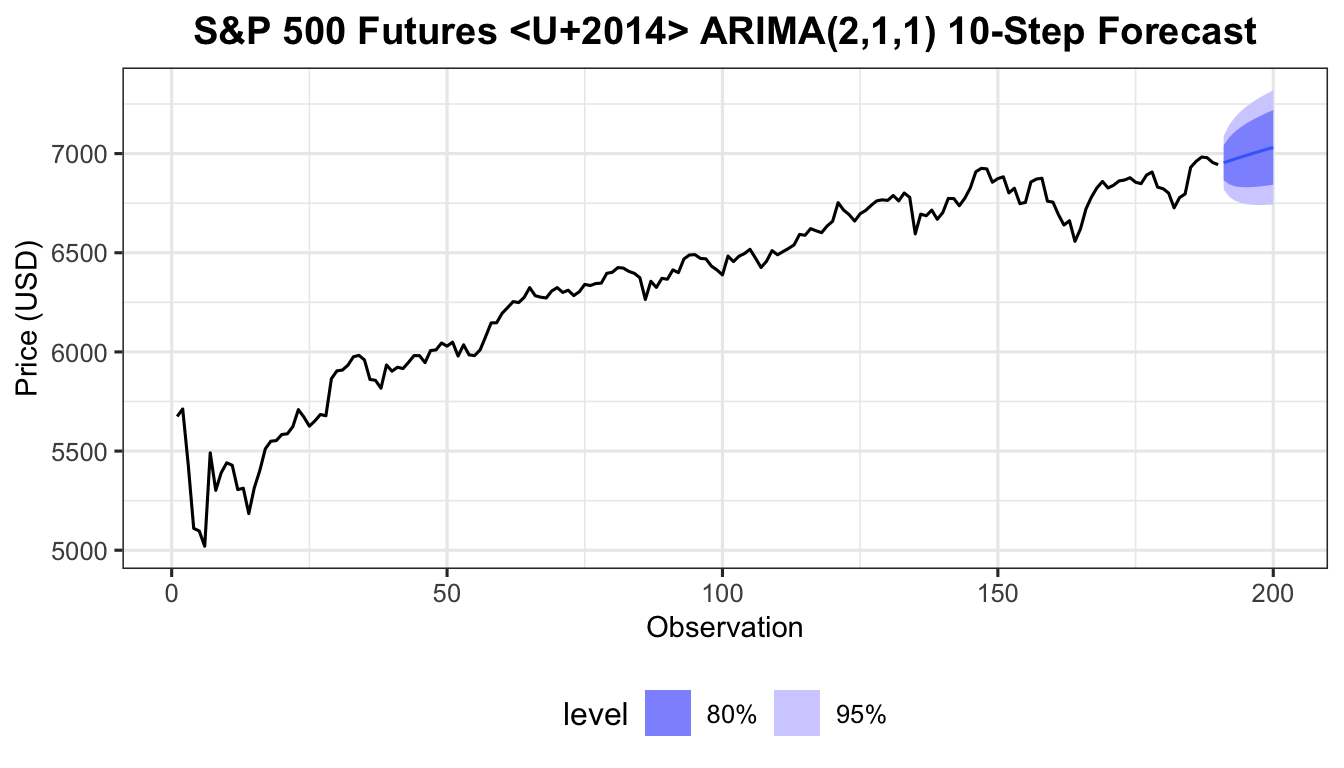

Figure 11: Ten-step-ahead forecast for the S&P 500 series. The model is refitted to the full available series before forecasting. Shaded bands show 80% and 95% prediction intervals.

7 Box-Jenkins: Seasonal ARIMA (SARIMA)

We now apply the full Box-Jenkins procedure to the Malaysia IPI Manufacturing Index (monthly, January 2015 to November 2025) — a series with both trend and seasonality.

7.1 Stage 1 — Model Identification (SARIMA)

The steps for SARIMA identification are:

Check for stationarity. If stationary → ARMA.
If not stationary, check for seasonality.
If seasonal → seasonal differencing: $z_t = y_t - y_{t-s}$.
If $z_t$ still not stationary → regular differencing: $w_t = z_t - z_{t-1}$.
Confirm stationarity with ADF test.
Determine $p$, $q$ (from ACF/PACF of $w_t$ at low lags) and $P$, $Q$ (from ACF/PACF at seasonal lags).

7.1.1 Data and Partition

Show R Code

# Estimation (first 82 obs) and evaluation (remaining) sets
n_total  <- length(ipi_ts)
sest     <- head(ipi_ts, 82)
seva     <- tail(ipi_ts, n_total - 82)

cat("Estimation set:", length(sest), "observations\n")

Estimation set: 82 observations

Show R Code

cat("Evaluation set:", length(seva), "observations\n")

Evaluation set: 49 observations

7.1.2 Step 1: Time Series Plot and Decomposition

Show R Code

autoplot(decompose(sest)) +
  labs(title = "Decomposition of IPI Manufacturing") +
  theme_ts()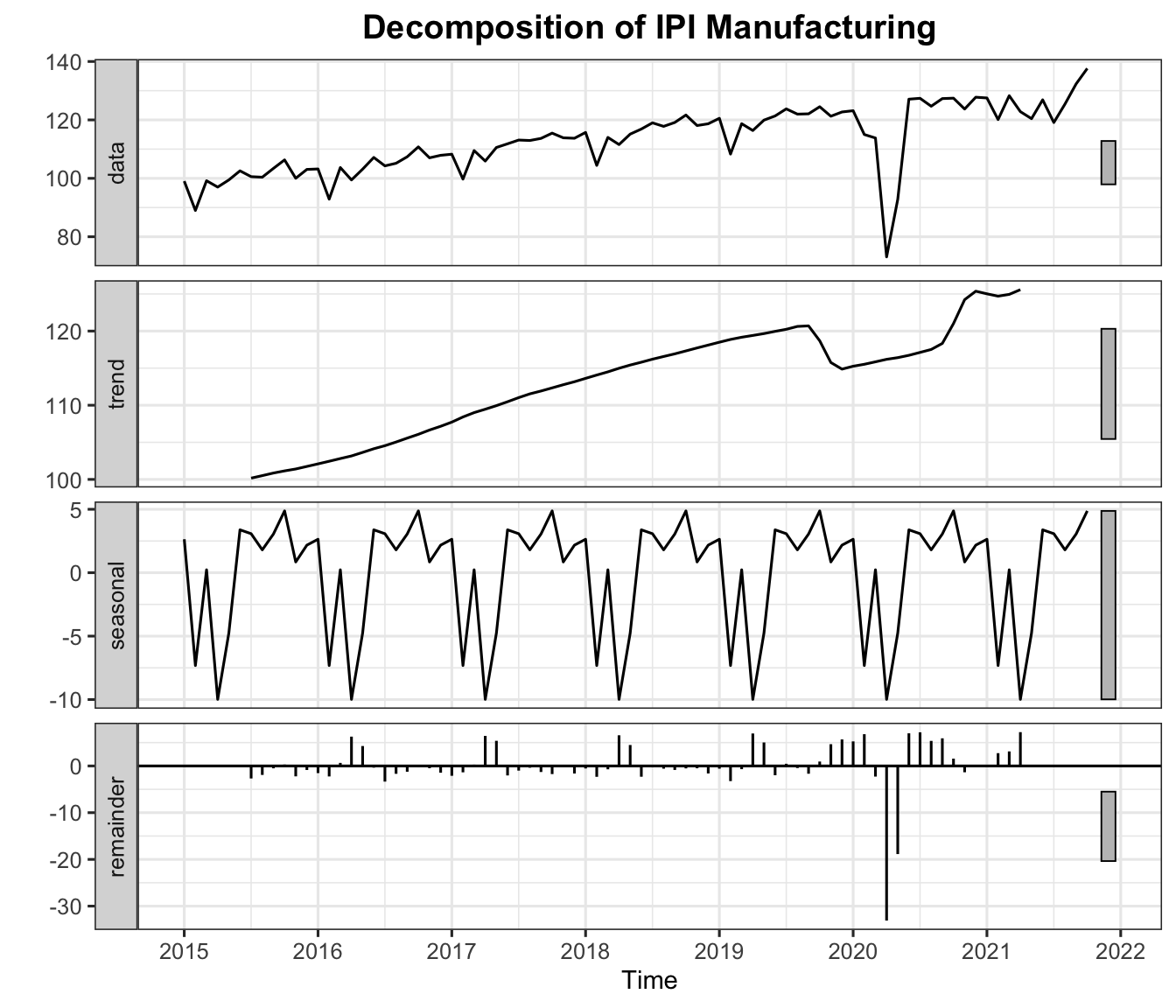

Figure 12: Classical decomposition of the IPI Manufacturing series. The seasonal component clearly repeats each year, confirming the need for seasonal differencing.

7.1.3 Step 2: ACF and ADF of Raw Series

Show R Code

ggAcf(sest, lag.max = 48) +
  labs(title = "ACF — IPI Estimation Set") +
  theme_ts()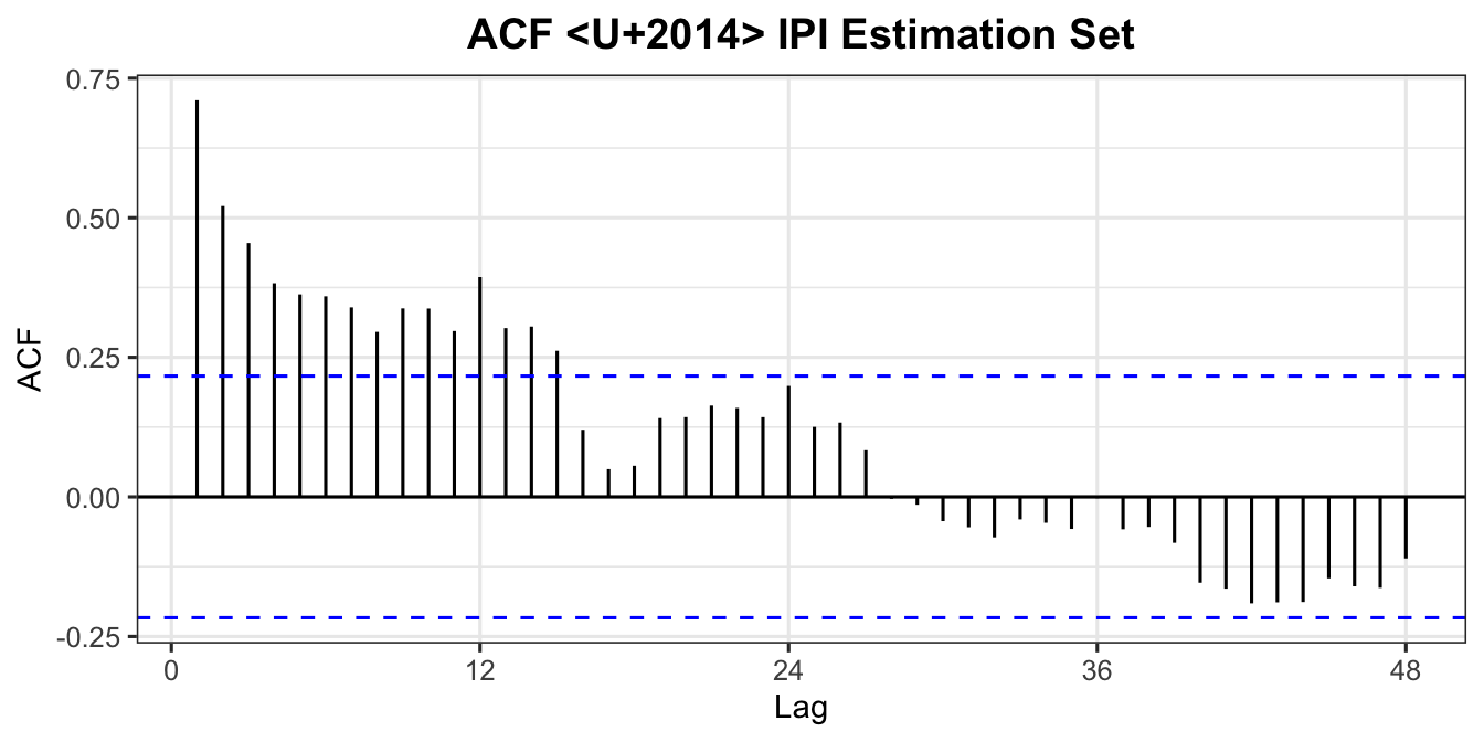

Figure 13: ACF of the IPI estimation set (up to 48 lags). The sinusoidal pattern with peaks at lags 12, 24, 36 indicates strong seasonality.

Show R Code

adf.test(sest)


    Augmented Dickey-Fuller Test

data:  sest
Dickey-Fuller = -3.9668, Lag order = 4, p-value = 0.0153
alternative hypothesis: stationary

Even if the ADF test indicates stationarity, the sinusoidal ACF pattern indicates a seasonal component — proceed with seasonal differencing.

7.1.4 Step 3: Seasonal Differencing

Show R Code

zt <- diff(sest, 12)

p_zt    <- autoplot(zt) +
  labs(title = expression("Seasonally Differenced IPI " ~ (z[t])),
       x = "Year", y = "") +
  theme_ts()
p_acfzt <- ggAcf(zt, lag.max = 48) +
  labs(title = "ACF — After Seasonal Differencing") +
  theme_ts()

grid.arrange(p_zt, p_acfzt, nrow = 2)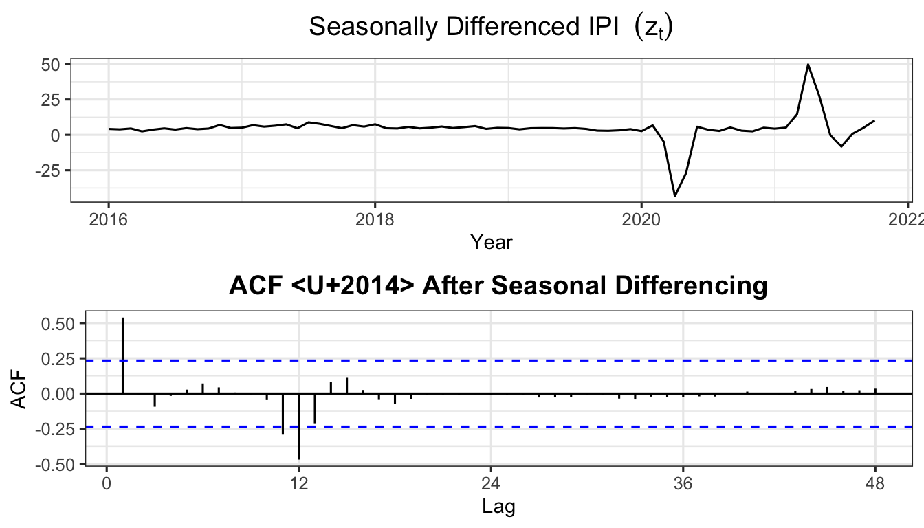

Figure 14: IPI after seasonal differencing ($z_t = y_t - y_{t-12}$). The seasonal pattern is substantially reduced.

Show R Code

adf.test(zt)


    Augmented Dickey-Fuller Test

data:  zt
Dickey-Fuller = -3.0054, Lag order = 4, p-value = 0.1664
alternative hypothesis: stationary

7.1.5 Step 4: Regular Differencing (if needed)

If the ADF test on $z_t$ still fails to reject $H_0$ ($p > 0.05$), apply a further first-order difference:

Show R Code

wt <- diff(zt, 1)

p_wt    <- autoplot(wt) +
  labs(title = expression("After Seasonal + Regular Differencing " ~ (w[t])),
       x = "Year", y = "") +
  theme_ts()
p_acfwt <- ggAcf(wt, lag.max = 48) +
  labs(title = "ACF — After Both Differences") +
  theme_ts()

grid.arrange(p_wt, p_acfwt, nrow = 2)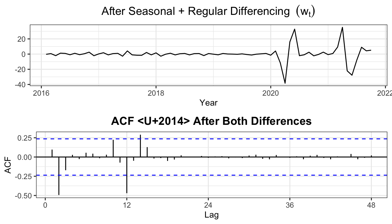

Figure 15: IPI after seasonal differencing followed by first-order differencing ($w_t = z_t - z_{t-1}$). The series fluctuates around zero with no trend or seasonal pattern — stationary.

Show R Code

adf.test(wt)


    Augmented Dickey-Fuller Test

data:  wt
Dickey-Fuller = -5.9055, Lag order = 4, p-value = 0.01
alternative hypothesis: stationary

7.1.6 Step 5: ACF and PACF for Order Determination

Show R Code

p_acf_w  <- ggAcf(wt,  lag.max = 48) +
  labs(title = "ACF — Stationary Series") + theme_ts()
p_pacf_w <- ggPacf(wt, lag.max = 48) +
  labs(title = "PACF — Stationary Series") + theme_ts()

grid.arrange(p_acf_w, p_pacf_w, ncol = 2)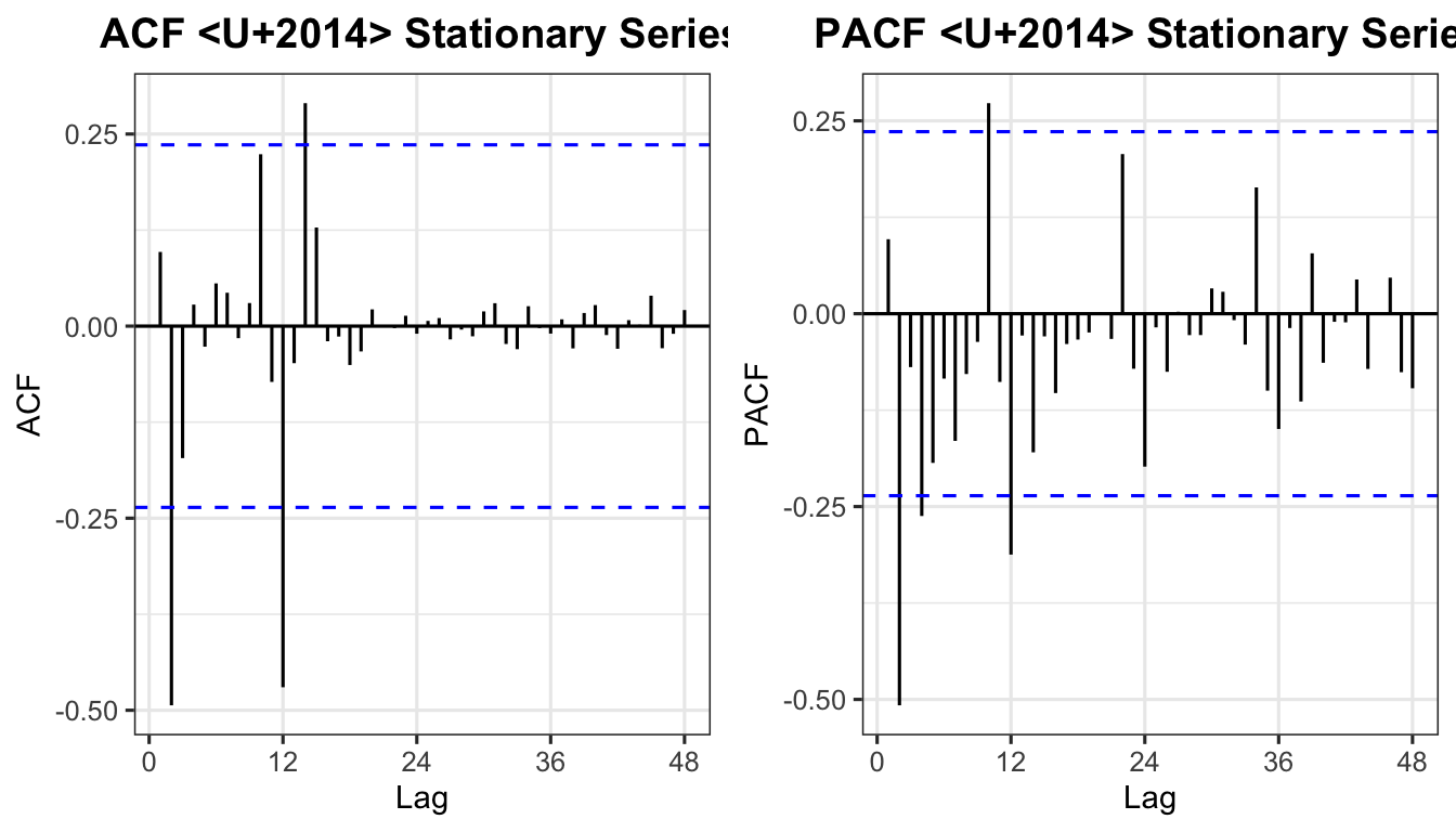

Figure 16: ACF (left) and PACF (right) of the fully differenced IPI series $w_t$. Significant spikes at low lags determine non-seasonal orders ($p$, $q$); significant spikes at seasonal lags 12, 24 determine seasonal orders ($P$, $Q$).

Reading the plots:

Plot	Significant spike location	Interpretation
ACF	Lag 1 (non-seasonal)	MA(1) → $q = 1$
ACF	Lag 12 (seasonal)	SMA(1) → $Q = 1$
PACF	Lag 1 (non-seasonal)	AR(1) → $p = 1$
PACF	Lag 12 (seasonal)	SAR(1) → $P = 1$

Suggested model: SARIMA$(1,1,1)(1,1,1)_{12}$

Competing models: SARIMA$(2,1,2)(1,1,1)_{12}$ and SARIMA$(1,1,0)(1,1,1)_{12}$

7.2 Stage 2 — Model Estimation (SARIMA)

Show R Code

sest_tbl <- as_tsibble(sest)
seva_tbl <- as_tsibble(seva)
ipi_tbl  <- as_tsibble(ipi_ts)

smodel1 <- sest_tbl |> model(ARIMA(value ~ pdq(1,1,1) + PDQ(1,1,1)))
smodel2 <- sest_tbl |> model(ARIMA(value ~ pdq(2,1,2) + PDQ(1,1,1)))
smodel3 <- sest_tbl |> model(ARIMA(value ~ pdq(1,1,0) + PDQ(1,1,1)))

report(smodel1)

Series: value 
Model: ARIMA(1,1,1)(1,1,1)[12] 

Coefficients:
          ar1     ma1     sar1     sma1
      -0.3961  0.6660  -0.0953  -0.7322
s.e.   0.2099  0.1593   0.3314   0.4365

sigma^2 estimated as 44.88:  log likelihood=-232.53
AIC=475.05   AICc=476.01   BIC=486.23

Estimated equation for SARIMA$(1,1,1)(1,1,1)_{12}$:

\[ (1 - \hat\phi_1 B)(1 - B)(1 - \hat\Phi_1 B^{12})(1 - B^{12})\,y_t = (1 + \hat\theta_1 B)(1 + \hat\Theta_1 B^{12})\,\varepsilon_t \tag{30} \]

Tip

Exercise: Write the estimated equations for:

SARIMA$(2,1,2)(1,1,1)_{12}$
SARIMA$(1,1,0)(1,1,1)_{12}$

7.3 Stage 3 — Model Validation (SARIMA)

7.3.1 ACF and PACF of Residuals

Show R Code

se1 <- residuals(smodel1)

p_ra  <- ggAcf(se1$.resid,  lag.max = 48) +
  labs(title = "Residual ACF")  + theme_ts()
p_rpa <- ggPacf(se1$.resid, lag.max = 48) +
  labs(title = "Residual PACF") + theme_ts()
grid.arrange(p_ra, p_rpa, ncol = 2)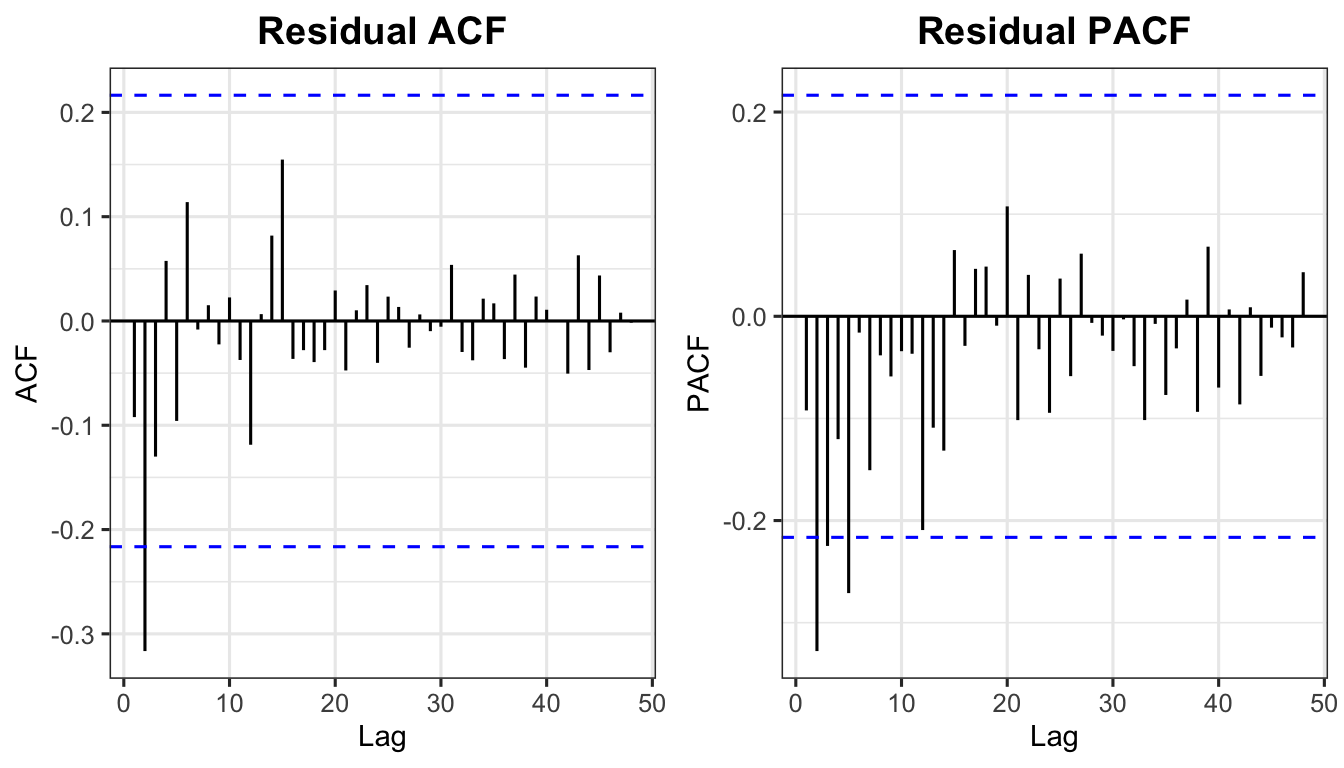

Figure 17: ACF (left) and PACF (right) of residuals from SARIMA$(1,1,1)(1,1,1)_{12}$. Residuals should have no significant spikes — confirming white noise.

7.3.2 Ljung-Box Test

The Box-Pierce statistic:

\[ Q_{\text{calc}} = (T - d)\sum_{k=1}^{h} r_k^2 \tag{31} \]

The Ljung-Box statistic (preferred for small samples):

\[ Q^*_{\text{calc}} = T(T+2)\sum_{k=1}^{h}\frac{r_k^2}{T-k} \tag{32} \]

Both are approximately $\chi^2$ distributed with $(h - p - q)$ degrees of freedom.

How many lags to use:

General rule: use $h = \sqrt{n}$ (e.g., $n=100 \Rightarrow h=10$)
Seasonal models: use $h = 2m$ where $m$ is the seasonal period (e.g., monthly $m=12 \Rightarrow h=24$)

Show R Code

Box.test(se1$.resid, lag = 24, type = "Ljung-Box", fitdf = 4)


    Box-Ljung test

data:  se1$.resid
X-squared = 19.067, df = 20, p-value = 0.5174

7.3.3 Model Comparison

Show R Code

# Ljung-Box p-values for all three models
lb_results <- data.frame(
  Model = c("SARIMA(1,1,1)(1,1,1)[12]",
            "SARIMA(2,1,2)(1,1,1)[12]",
            "SARIMA(1,1,0)(1,1,1)[12]"),
  p_value = c(
    Box.test(residuals(smodel1)$.resid, lag=24, type="Ljung-Box", fitdf=4)$p.value,
    Box.test(residuals(smodel2)$.resid, lag=24, type="Ljung-Box", fitdf=6)$p.value,
    Box.test(residuals(smodel3)$.resid, lag=24, type="Ljung-Box", fitdf=3)$p.value
  )
)
lb_results$Decision <- ifelse(lb_results$p_value > 0.05,
                              "Fail to reject H0", "Reject H0")
lb_results$Conclusion <- ifelse(lb_results$p_value > 0.05,
                                "White noise", "Not white noise")
print(lb_results)

                     Model   p_value          Decision  Conclusion
1 SARIMA(1,1,1)(1,1,1)[12] 0.5174481 Fail to reject H0 White noise
2 SARIMA(2,1,2)(1,1,1)[12] 0.9650902 Fail to reject H0 White noise
3 SARIMA(1,1,0)(1,1,1)[12] 0.1480511 Fail to reject H0 White noise

All models that pass the Ljung-Box test are candidate models. Select the best using AIC/BIC:

Show R Code

bind_rows(
  glance(smodel1) |> mutate(Model = "SARIMA(1,1,1)(1,1,1)[12]"),
  glance(smodel2) |> mutate(Model = "SARIMA(2,1,2)(1,1,1)[12]"),
  glance(smodel3) |> mutate(Model = "SARIMA(1,1,0)(1,1,1)[12]")
) |>
  select(Model, AIC, AICc, BIC) |>
  arrange(AIC)

# A tibble: 3 x 4
  Model                      AIC  AICc   BIC
  <chr>                    <dbl> <dbl> <dbl>
1 SARIMA(2,1,2)(1,1,1)[12]  457.  459.  473.
2 SARIMA(1,1,1)(1,1,1)[12]  475.  476.  486.
3 SARIMA(1,1,0)(1,1,1)[12]  478.  479.  487.

The model with the lowest AIC, AICc, and BIC is selected as the best model.

7.4 Stage 4 — Model Application: Forecasting (SARIMA)

Use the best model (refitted to the full IPI series) to generate a 12-step-ahead forecast:

Show R Code

# Identify best model (lowest AIC among those with white noise residuals)
best_sarima <- sest_tbl |> model(ARIMA(value ~ pdq(2,1,2) + PDQ(1,1,1)))

best_sarima |>
  refit(ipi_tbl) |>
  forecast(h = 12) |>
  autoplot(ipi_tbl, level = c(80, 95)) +
  labs(title = "Malaysia IPI Manufacturing — 12-Month Ahead Forecast",
       subtitle = "SARIMA(2,1,2)(1,1,1)[12]",
       x = "Year", y = "Index") +
  theme_ts()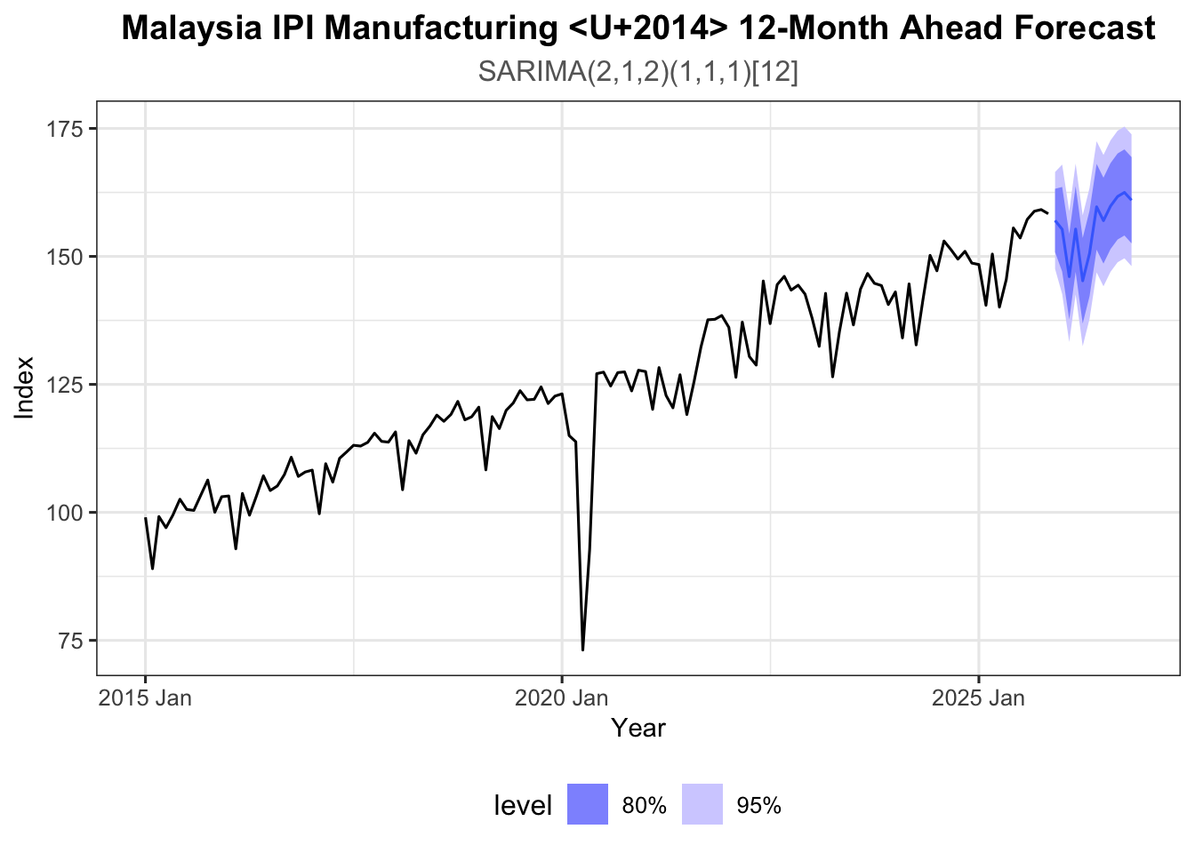

Figure 18: SARIMA forecast for IPI Manufacturing. The best model (selected by AIC/BIC) is refitted to the complete IPI series and used to forecast 12 months ahead. Shaded bands show 80% and 95% prediction intervals.

8 Summary

8.1 Box-Jenkins Methodology — Four Stages

Stage	Task	Tools
1 — Identification	Determine $p$, $d$, $q$ (and $P$, $D$, $Q$ for seasonal)	Time series plot, ACF, PACF, ADF test
2 — Estimation	Estimate model parameters	OLS, Maximum Likelihood (R: `ARIMA()`)
3 — Validation	Confirm residuals are white noise; select best model	Ljung-Box test, AIC, AICc, BIC
4 — Application	Generate point forecasts and prediction intervals	`forecast()`, confidence bands

8.2 ACF and PACF — Quick Reference

	ACF	PACF
AR($p$)	Tails off	Cuts off after lag $p$
MA($q$)	Cuts off after lag $q$	Tails off
ARMA($p$,$q$)	Tails off	Tails off
Non-stationary	Slow decay	Large at lag 1
Seasonal	Peaks at seasonal lags ($s$, $2s$, …)	Peaks at seasonal lags

8.3 Information Criteria Summary

Criterion	Formula	Penalty
AIC	$-2\log(L) + 2k$	Moderate
AICc	$\text{AIC} + \dfrac{2k(k+1)}{T-k-1}$	Moderate (small sample correction)
BIC	$-2\log(L) + k\log(T)$	Stronger (grows with $T$)

where $k = p + q + $ (1 if constant included, else 0).

9 References

Mohd Alias Lazim (2013). Introductory Business Forecasting: A Practical Approach (3rd ed.). UPENA, UiTM. ISBN: 978-983-3643.
Hyndman, R.J. and Athanasopoulos, G. (2018). Forecasting: Principles and Practice (2nd ed.). OTexts. Available at https://otexts.com/fpp2/.
Department of Statistics Malaysia. Industrial Production Index data retrieved from https://open.dosm.gov.my/data-catalogue.

1 Introduction

2 ARIMA Models

2.1 Autoregressive (AR) Model

2.1.1 AR(1) — the simplest form

2.2 Moving Average (MA) Model

2.2.1 MA(1) — the simplest form

2.3 Mixed Autoregressive Moving Average — ARMA(\(p\),\(q\))

2.3.1 ARMA(1,1) — the simplest form

2.4 Autoregressive Integrated Moving Average — ARIMA(\(p\),\(d\),\(q\))

2.4.1 ARIMA(1,1,1) — a simple case

2.5 Seasonal ARIMA — SARIMA(\(p\),\(d\),\(q\))(\(P\),\(D\),\(Q\))\(_s\)

2.5.1 Formulating SARIMA\((1,1,2)(1,1,1)_4\)

3 Box-Jenkins Methodology: Overview

4 Autocorrelation Function (ACF)

4.1 Definition

4.2 ACF of a Random Process (White Noise)

4.3 ACF of an AR(1) Process

4.4 ACF of an MA(1) Process

5 Partial Autocorrelation Function (PACF)

5.1 Definition

5.2 ACF and PACF Patterns — Model Identification Guide

5.2.1 Example: Constructing ACF and PACF Plots from a Table

6 Box-Jenkins: Non-Seasonal ARIMA

6.1 Stage 1 — Model Identification

6.1.1 Step 1a: Time Series Plot

6.1.2 Step 1b: ACF and PACF of the Raw Series

6.1.3 Step 1c: ADF Test on Raw Series

6.1.4 Step 1d: First-Order Differencing

6.1.5 Step 1e: ACF and PACF of Differenced Series

6.2 Stage 2 — Model Estimation (Non-Seasonal)

6.3 Stage 3 — Model Validation (Non-Seasonal)

6.3.1 Ljung-Box Test

6.3.2 Information Criteria

6.3.3 Parameter Redundancy

6.4 Stage 4 — Model Application: Forecasting (Non-Seasonal)

6.4.1 Three Steps for Point Forecasts

6.4.2 Forecast Exercise

6.4.3 Forecast Plot

7 Box-Jenkins: Seasonal ARIMA (SARIMA)

7.1 Stage 1 — Model Identification (SARIMA)

7.1.1 Data and Partition

7.1.2 Step 1: Time Series Plot and Decomposition

7.1.3 Step 2: ACF and ADF of Raw Series

7.1.4 Step 3: Seasonal Differencing

7.1.5 Step 4: Regular Differencing (if needed)

7.1.6 Step 5: ACF and PACF for Order Determination

7.2 Stage 2 — Model Estimation (SARIMA)

7.3 Stage 3 — Model Validation (SARIMA)

7.3.1 ACF and PACF of Residuals

7.3.2 Ljung-Box Test

7.3.3 Model Comparison

7.4 Stage 4 — Model Application: Forecasting (SARIMA)

8 Summary

8.1 Box-Jenkins Methodology — Four Stages

8.2 ACF and PACF — Quick Reference

8.3 Information Criteria Summary

9 References