Econometric modelling is a branch of economics that employs statistical methods to analyse economic phenomena, forecast future trends, and evaluate economic policies. It combines economic theory, mathematics, and statistical techniques to quantify and understand the relationships between economic variables.
Note
Econometric models go beyond univariate time series methods — they explain why a variable behaves as it does by relating it to other economic variables (its determinants). This gives forecasts a causal interpretation, which is valuable for policy analysis.
1.2 Purpose
Econometric models are used to:
Test economic theories and hypotheses.
Predict future economic variables and trends.
Assess the impact of policy changes or external shocks on the economy.
Make informed decisions in business, finance, and public policy.
1.3 Applications of Econometric Modelling
Application Area
Example
Macroeconomic Forecasting
Central banks forecast GDP growth, inflation, unemployment rates, and interest rates using large structural models.
Financial Markets
The Capital Asset Pricing Model (CAPM) and Arbitrage Pricing Theory (APT) estimate expected asset returns based on risk.
Labour Economics
Researchers use difference-in-differences and regression discontinuity designs to evaluate minimum wage laws.
Health Economics
Instrumental variables and propensity score matching address endogeneity in evaluating healthcare interventions.
Environmental Economics
Panel data and spatial econometrics assess the effectiveness of environmental regulations on economic growth.
Marketing & Consumer Behaviour
Discrete choice models and time series analysis forecast consumer demand and advertising effectiveness.
2 Basic Structure of Econometric Model
2.1 General Form
The variables used in econometric models are:
Dependent variable (\(y_t\)): the variable we want to explain or forecast.
Independent (explanatory) variables (\(x_{1t}, x_{2t}, \ldots, x_{mt}\)): the factors that help explain \(y_t\).
Equation (1) states that the level of \(y_t\) is influenced by the behaviour of variables \(x_{1t}, x_{2t}, \ldots, x_{mt}\), and the relationship is established from historical data.
\(\beta_i\) is the coefficient for the \(i\)-th independent variable,
\(\varepsilon_t\) is the error (disturbance) term at time \(t\),
The \(x_{it}\) matrix is assumed non-stochastic (fixed), and \(y_t\) is a random variable.
2.3 General Model with Lag Variables
A more general model, the Autoregressive Distributed Lag (ADL) model, allows both lagged values of the dependent variable and lagged values of the independent variables:
Including lagged values of \(y_t\) in the model is one of the most effective remedies for serial correlation. The ADL model is the foundation of the General-to-Specific modelling strategy covered later in this chapter.
3 Fundamental of OLS Technique
3.1 Ordinary Least Squares (OLS)
Ordinary Least Squares (OLS) is the standard method for estimating the parameters of a linear regression model. Its main objective is to minimise the sum of squared errors:
Solving these two normal equations simultaneously yields the OLS estimates \(\hat{\beta}_0\) and \(\hat{\beta}_1\).
Note
In practice, R’s lm() function performs all of these calculations internally using matrix algebra. Understanding the derivation helps you interpret what the function is doing under the hood and why the assumptions matter.
4 Issues in the Econometric Construction
4.1 Variable Selection Criteria
Variables included in the model must satisfy two conditions:
Statistical significance — the variable must have a meaningful statistical relationship with \(y_t\).
Theoretical (logical) justification — the relationship must be supported by economic theory.
Variable selection is the procedure of choosing a subset (from all possible subsets) of independent variables. The common criterion is to minimise the squared error while maintaining theoretical coherence.
4.1.1 Steps for Model Specification
Step
Description
Step 1
Identify the appropriate economic theory to select independent variables that explain the dependent variable.
Step 2
Ensure sufficient data are available. Rule of thumb: at least 5 observations per independent variable.
Step 3
Examine the relationships among variables using historical data to assess the general fitness of the model.
4.2 Model Cost
As model complexity increases, data requirements and computational costs increase.
More sophisticated models require more time, specialised software, and greater expertise.
A parsimonious model is preferred when it achieves comparable predictive performance at lower cost.
4.3 Model Complexity
Simple linear models are easy to interpret and visualise.
Models with many independent variables are difficult to envisage and may overfit the data.
Principle of parsimony: if two models have the same explanatory power, prefer the simpler one.
4.4 Future Values of Independent Variables
A key practical challenge in multi-variable forecasting:
To forecast \(y_{t+1}\), the analyst must also have (or forecast) \(x_{1(t+1)}\) and \(x_{2(t+1)}\).
Note
Challenge: If the future values of independent variables are themselves estimated with error, those errors propagate into the forecast of \(y\). This is a key limitation of econometric forecasting compared to univariate methods — more variables means more sources of forecast error.
5 Assumptions
5.1 Assumptions Pertaining to the Model
For OLS estimates to have desirable properties (unbiasedness, efficiency), the following model-level assumptions must hold:
Linearity — \(y_t\) is a linear function of the independent variables.
Correct specification — all relevant variables are included; no irrelevant variables are present.
No multicollinearity — the \(x_t\)’s must be mutually independent.
Sufficient sample size — the number of observations \(n\) must exceed the number of regressors \(m\).
5.2 Assumptions Pertaining to the Error Term
IID errors — the error terms \(\varepsilon_t\) are identically and independently distributed.
Homoscedasticity — \(\text{Var}(\varepsilon_t) = \sigma^2\) is constant for all \(t\).
No autocorrelation — \(\text{Cov}(\varepsilon_t, \varepsilon_s) = 0\) for all \(t \neq s\).
Exogeneity — the independent variables are uncorrelated with the error terms.
Drop the most insignificant variable (highest \(p\)-value) at each step — one at a time.
A variable may also be dropped if it registers the wrong sign contrary to theoretical expectations.
Repeat until all remaining variables are significant and pass all diagnostics.
Note
Why drop one variable at a time? The significance of one variable depends on what other variables are in the model. Dropping multiple variables simultaneously can lead to incorrect conclusions about which variables truly matter.
Practical considerations for the general model:
Maintain a small number of explanatory variables to control cost, avoid multicollinearity, and keep the model interpretable.
If multicollinearity exists, the offending variable (usually with the highest VIF) is a candidate for removal.
If the model is inadequate or mis-specified, add the next most promising variable (based on correlation with \(y_t\)).
Repeat until a well-specified model is obtained.
Note
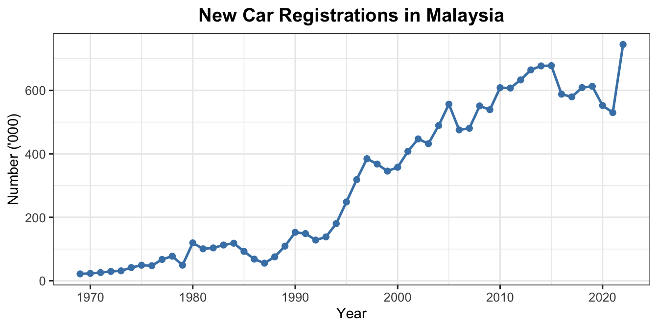
In this course, we primarily use the General-to-Specific approach, as illustrated in the worked example with Malaysian car registration data.
7 Statistical Validation and Testing Procedure
Failure to satisfy any of the following tests indicates that a model assumption is violated. Remedial action should then be taken: reformulate the model, include new variables, obtain more data, or apply variable transformations.
Test
Purpose
Decision Rule
F-test
Overall model fitness
If \(p < 0.05\), at least one variable is significant
t-test
Significance of each coefficient
If \(p < 0.05\), retain the variable
Adjusted \(R^2\)
Goodness of fit
Higher is better; preferred over \(R^2\)
Breusch-Pagan
Heteroscedasticity
If \(p > 0.05\), variances are constant (no problem)
Durbin-Watson
Serial correlation
DW \(\approx\) 2 and \(p > 0.05\) means no problem
VIF
Multicollinearity
VIF \(> 10\) indicates a serious problem
7.1 General Fitness (F-Test)
The F-test evaluates the overall significance of the model:
\(H_0\): All slope coefficients are zero (\(\beta_1 = \beta_2 = \cdots = \beta_m = 0\)).
\(H_1\): At least one coefficient is non-zero.
Decision: If the \(p\)-value from the F-test is less than 0.05, the model has overall fit and at least one variable is significant. Proceed to examine individual coefficients using t-tests. Otherwise, the model is considered poorly fit.
7.2 Regression Coefficients (t-Test)
After confirming the model is overall significant via the F-test, examine each individual coefficient \(\beta_1, \beta_2, \ldots, \beta_m\):
\(H_0\): \(\beta_i = 0\) (variable \(i\) has no effect on \(y\))
\(H_1\): \(\beta_i \neq 0\)
Decision: If \(p < 0.05\), retain the variable. Otherwise, consider removing it from the model.
7.3 Goodness of Fit (\(R^2\) and Adjusted \(R^2\))
The coefficient of determination\(R^2\) measures the proportion of total variation in \(y_t\) explained by the regression:
\(R^2 \in [0, 1]\), where 0 indicates no fit and 1 indicates perfect fit.
Problem with \(R^2\): It increases mechanically whenever a new variable is added, even if the variable adds no explanatory value. Therefore, use Adjusted \(R^2\):
where \(n\) is the number of observations and \(m\) is the number of independent variables. Adjusted \(R^2\) penalises for adding variables and is the preferred measure of goodness of fit.
7.4 Heteroscedasticity
Homoscedasticity means the variance of the error term is constant: \[\text{Var}(\varepsilon_t) = \sigma^2 \quad \text{for all } t\]
If this assumption is violated, the errors are heteroscedastic — their variance changes over time or across observations. Consequences:
OLS estimates are no longer the minimum variance (BLUE) estimators.
Standard errors and inference become unreliable.
Forecasts become less predictable as the forecast horizon extends.
Breusch-Pagan Test: - \(H_0\): Error variance is constant (homoscedastic). - \(H_1\): Error variance is non-constant (heteroscedastic). - Decision: If \(p > 0.05\), no heteroscedasticity problem. If \(p < 0.05\), heteroscedasticity is present — consider transforming the dependent variable (e.g., log transformation).
7.5 Serial Correlation (Autocorrelation)
The error terms must be uncorrelated across time: \[\text{Cov}(\varepsilon_t, \varepsilon_{t-s}) = 0 \quad \text{for all } s \neq 0\]
The most common form is first-order autocorrelation: \[\varepsilon_t = \rho \varepsilon_{t-1} + \nu_t \tag{17}\]
Since the variance of \(\varepsilon_t\)grows with \(k\), forecast accuracy deteriorates as the forecast horizon increases. When \(\rho = 0\), \(\text{Var}(\varepsilon_t) = \sigma^2_\varepsilon\) is constant and there is no serial correlation.
Decision: If the \(p\)-value from the Durbin-Watson test is less than 0.05, serial correlation is present.
Remedy: Include a lag of the dependent variable (\(y_{t-1}\)) or a lag of an independent variable. Usually, lag 1 is sufficient to resolve the problem.
7.6 Multicollinearity
Multicollinearity occurs when two or more independent variables are linearly related to each other.
The dataset contains 54 annual observations from 1969 to 2022. Based on economic theory, the expected relationships between each independent variable and new car registrations are:
Independent Variable
Expected Sign
Rationale
Unemployment Rate (%)
Negative
Higher unemployment reduces household income and car purchases
Higher per capita income directly boosts car demand
8.1.3 Creating the Lag Variable
Show R Code
# Create lag 1 of number of car registrations# This is needed to address serial correlation (see Model 2 onwards)lag1 <-c(NA, econ$`Number of Car Registration ('000)`[1:(length(econ$`Number of Car Registration ('000)`) -1)])
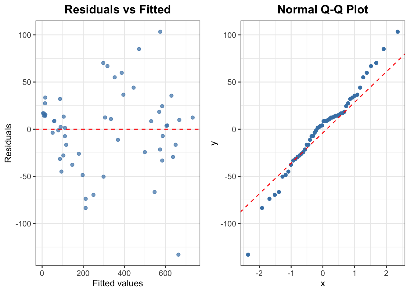
8.2 Model 1 — Full Model (All Variables, No Lag)
The first model includes all seven independent variables. This is the general model in the General-to-Specific procedure.
# Model 1: full model with all independent variables# Dependent variable Y: Number of Car Registration ('000)# Independent variables X: all economic predictorsmodel1 <-lm(`Number of Car Registration ('000)`~`Unemployment Rate (%)`+ CPI +`BLR (%)`+ GDP +`Total Export`+`Total Population`+ Income,data = econ)summary(model1)
Call:
lm(formula = `Number of Car Registration ('000)` ~ `Unemployment Rate (%)` +
    CPI + `BLR (%)` + GDP + `Total Export` + `Total Population` +
    Income, data = econ)

Residuals:
     Min       1Q   Median       3Q      Max
-133.033  -25.599    6.262   18.042  103.360

Coefficients:
                          Estimate Std. Error t value Pr(>|t|)
(Intercept)              1.108e+02  1.343e+02   0.825  0.41347
`Unemployment Rate (%)` -2.070e+01  7.653e+00  -2.705  0.00953 **
CPI                      4.406e-01  2.598e+00   0.170  0.86604
`BLR (%)`               -8.711e+00  6.251e+00  -1.394  0.17016
GDP                     -1.601e-09  1.156e-09  -1.385  0.17277
`Total Export`           1.768e+00  3.860e-01   4.579 3.55e-05 ***
`Total Population`       1.454e-05  6.130e-06   2.372  0.02192 *
Income                   3.715e-02  3.401e-02   1.092  0.28039
---
Signif. codes:  0 '***' 0.001 '**' 0.01 '*' 0.05 '.' 0.1 ' ' 1

Residual standard error: 46.27 on 46 degrees of freedom
Multiple R-squared:  0.9673,    Adjusted R-squared:  0.9623
F-statistic: 194.5 on 7 and 46 DF,  p-value: < 2.2e-16
Show R Code
# Diagnostic tests for Model 1cat("--- VIF (Multicollinearity) ---\n")
--- VIF (Multicollinearity) ---
Show R Code
vif(model1)
`Unemployment Rate (%)`                     CPI               `BLR (%)`
               3.849078                1.393722                7.000983
                    GDP          `Total Export`      `Total Population`
             414.470181               34.029012               54.943368
                 Income
             170.152327
Show R Code
cat("\n--- Durbin-Watson Test (Serial Correlation) ---\n")
--- Durbin-Watson Test (Serial Correlation) ---
Show R Code
durbinWatsonTest(model1)
 lag Autocorrelation D-W Statistic p-value
   1       0.4470231      1.101488       0
 Alternative hypothesis: rho != 0
Show R Code
cat("\n--- Breusch-Pagan Test (Heteroscedasticity) ---\n")
--- Breusch-Pagan Test (Heteroscedasticity) ---
Show R Code
bptest(model1)
    studentized Breusch-Pagan test

data:  model1
BP = 7.8119, df = 7, p-value = 0.3495
# Model 2: add lag1 to address serial correlationmodel2 <-lm(`Number of Car Registration ('000)`~`Unemployment Rate (%)`+ CPI +`BLR (%)`+ GDP +`Total Export`+`Total Population`+ Income + lag1,data = econ)summary(model2)
Call:
lm(formula = `Number of Car Registration ('000)` ~ `Unemployment Rate (%)` +
    CPI + `BLR (%)` + GDP + `Total Export` + `Total Population` +
    Income + lag1, data = econ)

Residuals:
    Min      1Q  Median      3Q     Max
-83.653 -14.255   0.009  13.669  94.445

Coefficients:
                          Estimate Std. Error t value Pr(>|t|)
(Intercept)              1.411e+02  1.094e+02   1.290 0.203828
`Unemployment Rate (%)` -1.473e+01  6.132e+00  -2.402 0.020587 *
CPI                      3.344e-01  2.154e+00   0.155 0.877331
`BLR (%)`               -4.880e+00  4.990e+00  -0.978 0.333483
GDP                     -9.560e-10  9.200e-10  -1.039 0.304454
`Total Export`           1.196e+00  3.232e-01   3.702 0.000593 ***
`Total Population`       3.357e-06  5.464e-06   0.614 0.542141
Income                   2.357e-02  2.693e-02   0.875 0.386057
lag1                     5.119e-01  9.389e-02   5.453 2.14e-06 ***
---
Signif. codes:  0 '***' 0.001 '**' 0.01 '*' 0.05 '.' 0.1 ' ' 1

Residual standard error: 36.48 on 44 degrees of freedom
  (1 observation deleted due to missingness)
Multiple R-squared:   0.98, Adjusted R-squared:  0.9764
F-statistic: 269.6 on 8 and 44 DF,  p-value: < 2.2e-16
cat("\n--- Durbin-Watson Test (Serial Correlation) ---\n")
--- Durbin-Watson Test (Serial Correlation) ---
Show R Code
durbinWatsonTest(model3)
 lag Autocorrelation D-W Statistic p-value
   1      0.03327008      1.751804   0.068
 Alternative hypothesis: rho != 0
Show R Code
cat("\n--- Breusch-Pagan Test (Heteroscedasticity) ---\n")
--- Breusch-Pagan Test (Heteroscedasticity) ---
Show R Code
bptest(model3)
    studentized Breusch-Pagan test

data:  model3
BP = 14.423, df = 7, p-value = 0.04416
Note
Model 3 Interpretation:
The model improved with higher \(R^2\) and no serial correlation problem.
However, CPI and Income registered incorrect signs.
Income is the most insignificant variable.
Action: Drop Income from the model.
8.5 Model 4 — Remove Income
Show R Code
# Model 4: remove Income (incorrect sign + most insignificant)model4 <-lm(`Number of Car Registration ('000)`~`Unemployment Rate (%)`+`BLR (%)`+`Total Export`+`Total Population`+ CPI + lag1,data = econ)summary(model4)
Call:
lm(formula = `Number of Car Registration ('000)` ~ `Unemployment Rate (%)` +
    `BLR (%)` + `Total Export` + `Total Population` + CPI + lag1,
    data = econ)

Residuals:
    Min      1Q  Median      3Q     Max
-79.452 -18.570  -0.189  12.885  99.914

Coefficients:
                          Estimate Std. Error t value Pr(>|t|)
(Intercept)              1.610e+02  9.250e+01   1.740 0.088530 .
`Unemployment Rate (%)` -1.420e+01  5.219e+00  -2.721 0.009169 **
`BLR (%)`               -3.609e+00  4.762e+00  -0.758 0.452389
`Total Export`           9.939e-01  2.588e-01   3.840 0.000374 ***
`Total Population`      -8.518e-07  3.540e-06  -0.241 0.810923
CPI                     -1.456e-01  2.080e+00  -0.070 0.944521
lag1                     5.297e-01  9.163e-02   5.781 6.17e-07 ***
---
Signif. codes:  0 '***' 0.001 '**' 0.01 '*' 0.05 '.' 0.1 ' ' 1

Residual standard error: 36.19 on 46 degrees of freedom
  (1 observation deleted due to missingness)
Multiple R-squared:  0.9794,    Adjusted R-squared:  0.9768
F-statistic: 365.1 on 6 and 46 DF,  p-value: < 2.2e-16
cat("\n--- Durbin-Watson Test (Serial Correlation) ---\n")
--- Durbin-Watson Test (Serial Correlation) ---
Show R Code
durbinWatsonTest(model4)
 lag Autocorrelation D-W Statistic p-value
   1      0.04457492      1.745045   0.086
 Alternative hypothesis: rho != 0
Show R Code
cat("\n--- Breusch-Pagan Test (Heteroscedasticity) ---\n")
--- Breusch-Pagan Test (Heteroscedasticity) ---
Show R Code
bptest(model4)
    studentized Breusch-Pagan test

data:  model4
BP = 13.282, df = 6, p-value = 0.03877
Note
Model 4 Interpretation:
The model produces a high \(R^2\) but most variables remain insignificant — a hallmark of multicollinearity.
Total Population has an incorrect sign (negative, contrary to the expected positive relationship) and is insignificant.
Action: Remove Total Population from the model.
8.6 Model 5 — Remove Total Population
Show R Code
# Model 5: remove Total Population (incorrect sign + insignificant)model5 <-lm(`Number of Car Registration ('000)`~`Unemployment Rate (%)`+`BLR (%)`+`Total Export`+ CPI + lag1,data = econ)summary(model5)
Call:
lm(formula = `Number of Car Registration ('000)` ~ `Unemployment Rate (%)` +
    `BLR (%)` + `Total Export` + CPI + lag1, data = econ)

Residuals:
    Min      1Q  Median      3Q     Max
-81.417 -17.893   0.529  12.971  98.928

Coefficients:
                         Estimate Std. Error t value Pr(>|t|)
(Intercept)             146.07589   68.07994   2.146   0.0371 *
`Unemployment Rate (%)` -13.82127    4.92741  -2.805   0.0073 **
`BLR (%)`                -3.49417    4.69007  -0.745   0.4600
`Total Export`            0.95831    0.21034   4.556 3.71e-05 ***
CPI                       0.03282    1.92420   0.017   0.9865
lag1                      0.52062    0.08273   6.293 9.67e-08 ***
---
Signif. codes:  0 '***' 0.001 '**' 0.01 '*' 0.05 '.' 0.1 ' ' 1

Residual standard error: 35.82 on 47 degrees of freedom
  (1 observation deleted due to missingness)
Multiple R-squared:  0.9794,    Adjusted R-squared:  0.9772
F-statistic: 447.1 on 5 and 47 DF,  p-value: < 2.2e-16
cat("\n--- Durbin-Watson Test (Serial Correlation) ---\n")
--- Durbin-Watson Test (Serial Correlation) ---
Show R Code
durbinWatsonTest(model6)
 lag Autocorrelation D-W Statistic p-value
   1      0.05149487      1.734734    0.15
 Alternative hypothesis: rho != 0
Show R Code
cat("\n--- Breusch-Pagan Test (Heteroscedasticity) ---\n")
--- Breusch-Pagan Test (Heteroscedasticity) ---
Show R Code
bptest(model6)
    studentized Breusch-Pagan test

data:  model6
BP = 11.858, df = 4, p-value = 0.01844
Note
Model 6 Interpretation:
After removing CPI, the model improved significantly: high \(R^2\) with three significant variables.
The Durbin-Watson value confirms no serial correlation problem.
However, VIF values for Total Export and the lag variable indicate multicollinearity still exists between these two variables.
Action: Remove Total Export from the model.
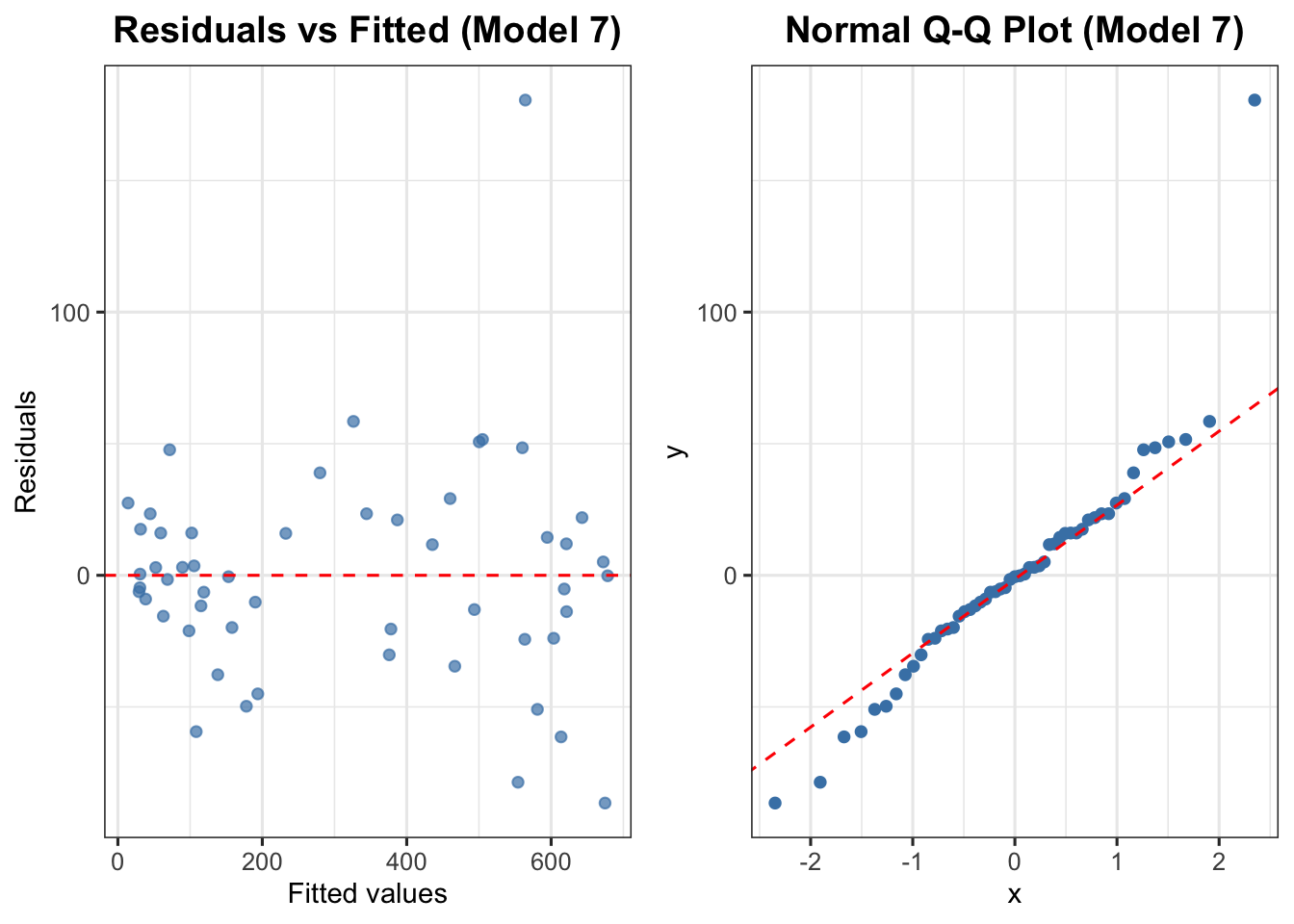
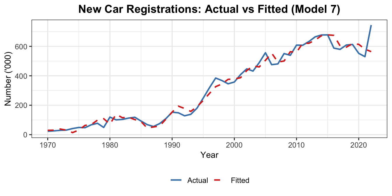
8.8 Model 7 — Final Model (Remove Total Export)
Show R Code
# Model 7: final model — remove Total Export# Remaining variables: Unemployment Rate, BLR, lag1model7 <-lm(`Number of Car Registration ('000)`~`Unemployment Rate (%)`+`BLR (%)`+ lag1,data = econ)summary(model7)
Call:
lm(formula = `Number of Car Registration ('000)` ~ `Unemployment Rate (%)` +
    `BLR (%)` + lag1, data = econ)

Residuals:
    Min      1Q  Median      3Q     Max
-86.523 -20.412  -0.523  17.512 180.560

Coefficients:
                         Estimate Std. Error t value Pr(>|t|)
(Intercept)             264.93628   74.43585   3.559 0.000838 ***
`Unemployment Rate (%)` -16.68328    5.77138  -2.891 0.005715 **
`BLR (%)`               -13.84240    4.75453  -2.911 0.005402 **
lag1                      0.78071    0.06949  11.235 3.66e-15 ***
---
Signif. codes:  0 '***' 0.001 '**' 0.01 '*' 0.05 '.' 0.1 ' ' 1

Residual standard error: 42.31 on 49 degrees of freedom
  (1 observation deleted due to missingness)
Multiple R-squared:  0.9701,    Adjusted R-squared:  0.9682
F-statistic: 529.2 on 3 and 49 DF,  p-value: < 2.2e-16
\(\hat{y}_t\) = estimated number of new car registrations (’000) in year \(t\),
\(x_{1t}\) = Unemployment Rate (%) in year \(t\),
\(x_{2t}\) = Base Lending Rate, BLR (%) in year \(t\),
\(y_{t-1}\) = lag 1 of new car registrations (’000).
8.9.1 Interpretation of Coefficients
Coefficient
Value
Interpretation
Intercept
264.94
Baseline car registrations when all predictors are zero
Unemployment Rate
\(-16.68\)
A 1 percentage-point increase in unemployment reduces car demand by approximately 16,680 units
BLR
\(-13.84\)
A 1 percentage-point increase in BLR reduces car demand by approximately 13,840 units
Lag of car registrations
\(+0.78\)
If car registrations increased by 1,000 last year, demand this year increases by approximately 780 units
All signs are consistent with economic theory: higher unemployment and higher borrowing costs both suppress consumer demand for cars, while past registration levels exhibit strong positive persistence.
8.10 Forecasting with the Final Model
8.10.1 Point Forecast for 2023
Given:
Unemployment Rate for 2023: \(x_{1,2023} = 3.3\%\)
BLR for 2023: \(x_{2,2023} = 6.89\%\)
Number of car registrations in 2022: \(y_{2022} = 744.78\) (’000)
Show R Code
# Extract coefficients from the final modelcoefs <-coef(model7)cat("Model coefficients:\n")
# Future values of independent variables for 2023unemp_2023 <-3.3# Unemployment Rate (%)blr_2023 <-6.89# BLR (%)y_2022 <-744.78# Car registrations in 2022 ('000)# One-step-ahead forecasty_hat_2023 <- coefs["(Intercept)"] + coefs["`Unemployment Rate (%)`"] * unemp_2023 + coefs["`BLR (%)`"] * blr_2023 + coefs["lag1"] * y_2022cat("\nForecast for 2023 (number of new car registrations, '000):",round(y_hat_2023, 2), "\n")
Forecast for 2023 (number of new car registrations, '000): 695.96
Show R Code
cat("Forecast in actual units:", round(y_hat_2023 *1000), "\n")
Forecast in actual units: 695961
Note
Forecasting caveat: The quality of this forecast depends on how accurately we know (or can forecast) the unemployment rate and BLR for 2023. If those values are themselves uncertain, the forecast error will be larger than the model’s in-sample statistics suggest.
Table 2: Summary of all models in the General-to-Specific procedure
Model
Change from Previous
Adj. R<U+00B2>
DW p-value
BP p-value
Model 1
None (full model)
0.9623
0.000
0.349
Model 2
<U+2014> (add lag1)
0.9764
0.156
0.020
Model 3
GDP removed
0.9763
0.082
0.044
Model 4
Income removed
0.9768
0.110
0.039
Model 5
Total Population removed
0.9772
0.122
0.033
Model 6
CPI removed
0.9777
0.176
0.018
Model 7
Total Export removed
0.9682
0.194
0.220
9 Summary
This chapter covered the complete framework for econometric modelling in time series forecasting. The key takeaways are:
Model Structure: Econometric models relate a dependent variable to multiple independent (explanatory) variables, grounded in economic theory. The ADL model incorporates both current and lagged variables.
OLS Estimation: Ordinary Least Squares minimises the sum of squared residuals. Understanding its derivation helps interpret model output and diagnose problems.
Issues in Model Construction: Variable selection must balance statistical significance with theoretical justification. Practical challenges include model cost, complexity, and the need for future values of predictors.
Assumptions: Five key assumptions govern OLS — linearity, correct specification, no multicollinearity, homoscedasticity, and no serial correlation. Violations require diagnostic tests and remedial action.
Model Estimation Strategies:
General-to-Specific (backward): Start with the full model and systematically drop the most insignificant variable at each stage until a parsimonious model is reached.
Specific-to-General (forward): Start simple and add variables one at a time.
Statistical Validation: A valid model must pass six diagnostic tests: F-test, t-tests, adjusted \(R^2\), Breusch-Pagan (heteroscedasticity), Durbin-Watson (serial correlation), and VIF (multicollinearity).
Worked Example: The final model for Malaysian new car registrations identified Unemployment Rate, BLR, and the lag of car registrations as the significant determinants. The model satisfies all diagnostic conditions and produces an interpretable, parsimonious equation.
10 References
Mohd Alias Lazim (2013). Introductory Business Forecasting: A Practical Approach, 3rd ed. UPENA, UiTM. ISBN: 978-983-3643.